Visualization Tear Sheets
TearSheet is the visualization class for the pairs analysis process based on different modules implemented in the ArbitrageLab package. It creates a locally ran Flask server, bringing an interactive approach to the data visualization with Plotly’s Dash.
Note
Running run_server() will produce the warning
“Warning: This is a development server. Do not use app.run_server in production, use a production WSGI server like gunicorn instead.”
However, this is okay and the Dash server will run without a problem.
Currently, two tear sheets are present in the module: Cointegration analysis and OU-model analysis available for the users.
Cointegration Tear Sheet
Note
All the methods used in the creation of this tear sheet are available in the arbitragelab.cointegration_approach module.
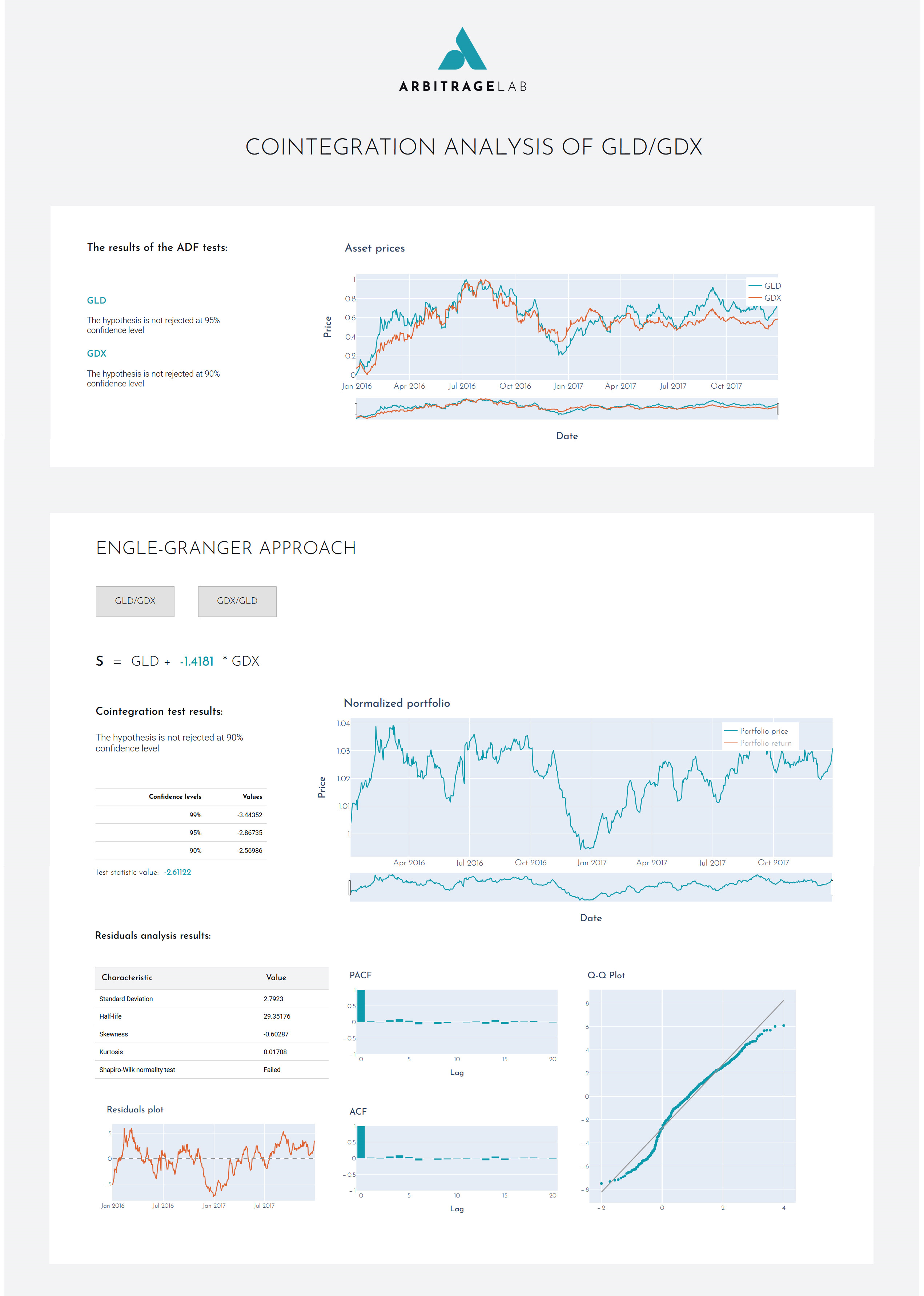
The first section contains the ADF test results for each of the assets from the provided pair separately and a plot of their normalized price series.
The second section is dedicated to the Engle-Granger cointegration test and further analysis. The results are provided for both possible combinations of the assets in the Engle-Granger-type portfolio and you can switch between them by clicking a respective button.
Provided data:
Portfolio coefficient
Cointegration test results
Normalized portfolio price/returns plot
Model residuals analysis
Statistical characteristics
Residuals plot
ACF and PACF plots
Q-Q plot
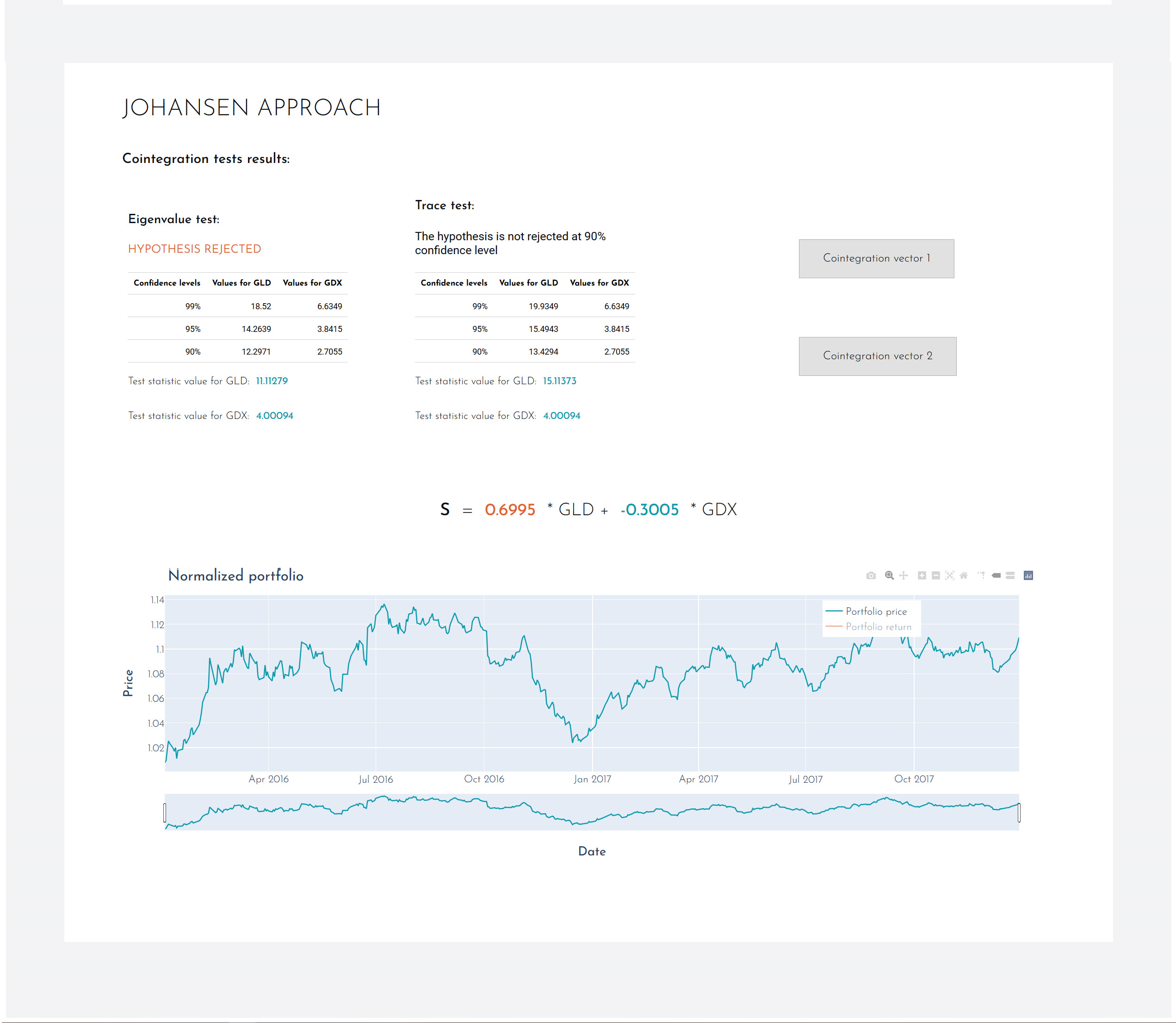
The third section is focused on the Johansen cointegration test and further portfolio analysis. The results are provided for both possible cointegration vectors of the assets in the Johansen-type portfolio, and you can switch between them by clicking a respective button.
Provided data:
Cointegrated portfolio coefficients
Cointegration test results for both eigen and trace cointegration tests
Normalized portfolio price/returns plot
Implementation
Code Example
# Import ArbitrageLab tools
from arbitragelab.tearsheet import TearSheet

# Initialize TearSheet class
tearsheet = TearSheet()

# Get server app
server = tearsheet.cointegration_tearsheet(data)

# Run server
server.run_server(port=8050)
OU Model Tear Sheet
Note
All the methods used in the creation of this tear sheet are availible in the arbitragelab.optimal_mean_reversion module.
The first section contains the information regarding the cointegration of the provided assets and also parameters of the fitted OU model to created optimal spread. The results are provided for both possible combination of the assets in the Engle-Granger-type portfolio, and you can switch between them by clicking the respective button.
Provided data:
Optimal portfolio coefficient
Cointegration test results for the two assets
Normalized portfolio price/returns plot
Fitted OU process characteristics
Spread price
Simulated OU process with the same parameters
The second section serves as a testing ground for the optimal stopping and liquidation levels calculation. The user is invited to alter the values of the discount rate, transaction cost, or set a stop-loss level - if optimal solutions exist, all the changes will be reflected onto the optimal levels graph.
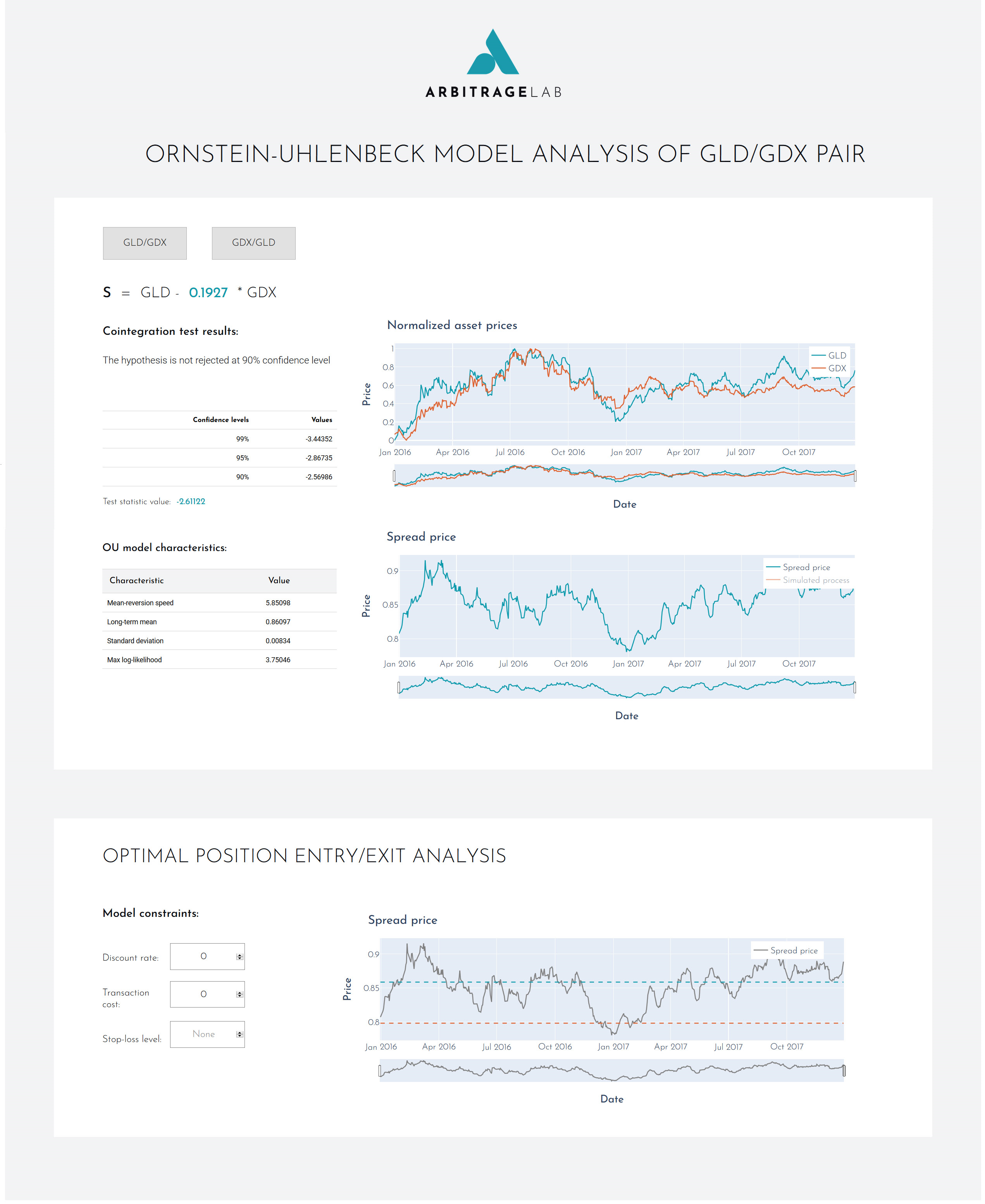
Note
The optimal levels graph may appear blank or unchanging after new parameters have been entered, since it takes time for the model to be retrained. However, they will load eventually.
Implementation
Code Example
# Import ArbitrageLab tools
from arbitragelab.tearsheet import TearSheet

# Initialize TearSheet class
tearsheet = TearSheet()

# Get server app
server = tearsheet.ou_tearsheet(data)

# Run server
server.run_server(port=8050)
Running Dash in Jupyter
You can easily run a Dash server within Jupyter Notebook. The Jupyter Dash library is used to provide this functionality.
When you initialize the server by using either cointegration_tearsheet or ou_tearsheet functions, you must add argument app_display='jupyter'.
Warning
Jupyter layout may not be optimal for all devices as it depends on the screen ratio, resolution and scaling.
To run the visualizations in Jupyter, replace:
# Import ArbitrageLab tools
from arbitragelab.tearsheet import TearSheet

# Initialize TearSheet class
tearsheet = TearSheet()

# Get server app
server = tearsheet.cointegration_tearsheet(data)

# Run server
server.run_server(port=8050)
With:
# Import ArbitrageLab tools
from arbitragelab.tearsheet import TearSheet

# Initialize TearSheet class
tearsheet = TearSheet()

# Get server app with extra argument 'jupyter'
server = tearsheet.cointegration_tearsheet(data, app_display='jupyter')

# Run server
server.run_server(mode='inline', port=8050)
Initialising the server with an additional argument 'jupyter', creates a JuptyerDash class instead of a Dash class.
Running mode='inline' will allow the interactive visualisations to display within a cell output of the Jupyter notebook.
For detailed explanations of the different modes, refer to
this article on Jupyter Dash.