Note
The following implementations and documentation closely follow the work of Tim Leung: Tim Leung and Xin Li Optimal Mean reversion Trading: Mathematical Analysis and Practical Applications.
Trading Under the Ornstein-Uhlenbeck Model
Warning
Alongside with Leung’s research we are using \(\theta\) for mean and \(\mu\) for mean-reversion speed, while other sources e.g. Wikipedia, use \(\theta\) for mean reversion speed and \(\mu\) for mean.
Model fitting
Note
We are solving the optimal stopping problem for a mean-reverting portfolio that is constructed by holding \(\alpha = \frac{A}{S_0^{(1)}}\) of a risky asset \(S^{(1)}\) and shorting \(\beta = \frac{B}{S_0^{(2)}}\) of another risky asset \(S^{(2)}\), yielding a portfolio value:
Since in terms of mean-reversion we care only about the ratio between \(\alpha\) and \(\beta\), without the loss of generality we can set \(\alpha = const\) and A = $1, while varying \(\beta\) to find the optimal strategy \((\alpha,\beta^*)\)
We establish Ornstein-Uhlenbeck process driven by the SDE:
\(\theta\) − long term mean level, all future trajectories of 𝑋 will evolve around a mean level 𝜃 in the long run.
\(\mu\) - speed of reversion, characterizes the velocity at which such trajectories will regroup around \(\theta\) in time.
\(\sigma\) - instantaneous volatility, measures instant by instant the amplitude of randomness entering the system. Higher values imply more randomness.
Under the OU model the probability density function of \(X_t\) with increment \(\Delta t = t_i - t_{i-1}\) is:
Warning
The following algorithms are devised and best suited for the data frequencies ranging from yearly to daily. Usage of the intraday data is theoretically possible, but as the value of time increment \(\Delta t\) becomes closer to zero, it might lead to divergence in the optimization process.
We observe the resulting portfolio values \((x_i^\beta)_{i = 0,1,\cdots,n}\) for every strategy \(\beta\) realized over an n-day period. To fit the model to our data and find optimal parameters we define the average log-likelihood function:
Then, maximizing the log-likelihood function by applying maximum likelihood estimation(MLE) we are able to determine the parameters of the model and fit the observed portfolio prices to an OU process. Let’s denote the maximized average log-likelihood by \(\hat{\ell}(\theta^*,\mu^*,\sigma^*)\). Then for every \(\alpha\) we choose \(\beta^*\), where:
Optimal Timing of Trades
Suppose the investor already has a position with a value process \((X_t)_{t>0}\) that follows the OU process. When the investor closes his position at the time \(\tau\) he receives the value \((X_{\tau})\) and pays a constant transaction cost \(c_s \in \mathbb{R}\) To maximize the expected discounted value we need to solve the optimal stopping problem:
where \(T\) denotes the set of all possible stopping times and \(r > 0\) is our subjective constant discount rate. \(V(x)\) represents the expected liquidation value accounted with X.
Current price plus transaction cost constitute the cost of entering the trade and in combination with \(V(x)\) we can formalize the optimal entry problem:
with
To sum up this problem, we, as an investor, want to maximize the expected difference between the current price of the position - \(x_{\nu}\) and its’ expected liquidation value \(V(X_{\nu})\) minus transaction cost \(c_b\)
Note
Following part of the chapter presents the analytical solution for the optimal stopping problem, both the default version and the version with the inclusion of the stop-loss level.
To solve this problem we denote the OU process infinitesimal generator:
and recall the classical solution of the differential equation
Then we are able to formulate the following theorems
(proven in Optimal Mean reversion Trading: Mathematical Analysis and Practical Applications by Tim Leung and Xin Li) to provide the solutions to following problems:
Default optimal stopping problem
Theorem 2.6 (p.23):
The optimal liquidation problem admits the solution:
The optimal liquidation level \(b^*\) is found from the equation:
Corresponding optimal liquidation time is given by
Theorem 2.10 (p.27):
The optimal entry timing problem admits the solution:
The optimal entry level \(d^*\) is found from the equation:
Where “\(\hat{\ }\)” represents the use of transaction cost and discount rate of entering.
Optimal stopping problem with stop-loss
When we include the stop-loss in our optimal stopping problems the theorems we use to find the solution are:
Theorem 2.13 (p.31):
The optimal liquidation problem admits the solution:
The optimal liquidation level \(b_L^*\) is found from the equation:
Corresponding optimal liquidation time is given by
Helper functions C and D defined as following:
Theorem 2.42 (p.35):
The optimal entry timing problem admits the solution:
The optimal entry interval \((a_L^*,d_L^*)\) is found using the respective equations:
How to use this submodule
This module gives you the ability to calculate optimal values of entering and liquidating the position for your portfolio. The whole process takes only 2 steps.
Step 1: Model fitting
In this step we need to use fit function to fit OU model to our training data and set the constant
parameters like transaction costs, discount rates, stop-loss level and data frequency. You have a choice not
to set the stop-loss level at the beginning, but it will deny access to the functions that use the stop-loss level.
To access them you just need to set the parameter self.L. Also there is a possibility to not use the whole
provided training sample, limiting it to a time interval of your choice with start and end parameters.
That option can be used if you provide a pandas DataFrame as an input data with Datetime-type indices. You can also use an np.array of two time series of asset prices, and the optimal portfolio will be constructed by the function itself, or use your own portfolio values as an input data.
Implementation
Tip
To retrain the model just use one of the functions fit_to_portfolio or fit_to_assets.
You have a choice either to use the new dataset or to change the training time interval of your currently
used dataset.
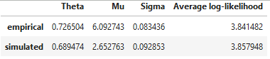
It is important to understand how good of a fit your data is compared to a simulated process with the
same parameters. To check we can use check_fit function that shows the optimal parameter values obtained
by fitting the OU model to our data and from the OU model simulated using our fitted parameters.
Tip
If you are interested in data generation you can create OU process simulations
using the ou_model_simulation function. The parameters used for the
model can be either the fitted parameters to your data or you can set all of them
for yourself.
Since the half-life of the OU process parameter is widely used in various researches, the module has a function for calculating its value.
Step 2: Determining the optimal entry and exit values
To get the optimal liquidation or entry level for your data we need to call one of the functions mentioned below. They present the solutions to the equations established during the theoretical part. To choose whether to account for stop-loss level or not choose the respective set of functions.
Implementation
\(b^*\): - optimal level of liquidation:
\(d^*\) - optimal level of entry:
\(b_L^*\) - optimal level of liquidation, accounting for preferred stop-loss level:
\([a_L^*,d_L^*]\) - optimal level of entry, accounting for preferred stop-loss level:
Tip
General rule for the use of the optimal levels:
If not bought, buy the portfolio as soon as portfolio price reaches the optimal entry level (enters the interval).
If bought, liquidate the position as soon as portfolio price reaches the optimal liquidation level.
Step 3: (Optional) Plot the optimal levels on your data
Additionally you have the ability to plot your optimal levels onto your out-of-sample data. Similarly to the fit step you have a choice whether to use portfolio prices or an array of asset prices. In the case of the latter optimal coefficient found during the fit stage will be used to create a portfolio.

Implementation
Tip
To view al the model stats, including the optimal levels call the description function

Example
As data we will use downloaded GLD and GDX tickers from Yahoo Finance.
import numpy as np
import pandas as pd
import yfinance as yf

# Import data from Yahoo finance
data1 =  yf.download("GLD GDX", start="2012-03-25", end="2016-01-09")
data2 =  yf.download("GLD GDX", start="2016-02-21", end="2020-08-15")

# You can use the pd.DataFrame of two asset prices
data_train_dataframe = data1["Adj Close"][["GLD", "GDX"]]

# And also we can create training dataset as an array of two asset prices
data_train = np.array(data1["Adj Close"][["GLD", "GDX"]])

# Create an out-of-sample dataset
data_oos = data2["Adj Close"][["GLD", "GDX"]]
The following examples show how the described above module can be used on real data:
Example 1
In this example we are using pd.DataFrame as an input data for the model. We train our model
on the whole provided sample and showcase our results on the separate out-of-sample dataset. We also include the
stop-loss level in this example.
from arbitragelab.optimal_mean_reversion import OrnsteinUhlenbeck

# Create the class object
example = OrnsteinUhlenbeck()

# Fit the model to the training data and allocate data frequency,
# transaction costs, discount rates and stop-loss level

# Chosen data type can be pd.DataFrame
example.fit(data_train_dataframe, data_frequency="D", discount_rate=[0.05, 0.05],
            transaction_cost=[0.02, 0.02], stop_loss=0.2)

# Check the model fit
print(example.check_fit())

# Showcase the data for both variations of the problem on the out of sample data
fig = example.plot_levels(data_oos, stop_loss=True)
fig.set_figheight(15)
fig.set_figwidth(10)
Example 2
In this example we are using pd.DataFrame as an input data for the model. We train our model
on the slice of the provided data chosen based on provided time interval and showcase our results with
description function. We include the stop-loss level in this example and change it manually
along the way. In the end we chose to retrain our data on a different slice of the provided data chosen
based on provided time interval.
from arbitragelab.optimal_mean_reversion import OrnsteinUhlenbeck

# Create the class object
example = OrnsteinUhlenbeck()

# Fit the model to the training data and allocate data frequency,
# transaction costs, discount rates and stop-loss level

# We can specify the interval we want to use for training
example.fit(data_train_dataframe, data_frequency="D", discount_rate=[0.05, 0.05],
            start="2012-03-27", end="2013-12-08",
            transaction_cost=[0.02, 0.02], stop_loss=0.2)

# Check the model fit
print(example.check_fit(),"\n")

# Stop-loss level, transaction costs and discount rates
# can be changed along the way
example.L = 0.3

# Call the description function to see all the model's parameters and optimal levels
print("Model description:\n",example.description())

# Retrain the model

# By changing the training interval
example.fit_to_assets(start="2015-08-25", end="2016-12-09")
Example 3
In this example we are using np.array as an input data for the model. We train our model
on the whole provided array and showcase our results on separate out-of-sample data. We don’t include the
stop-loss level in this example. In the end we chose to retrain our data on an out-of-sample dataset.
from arbitragelab.optimal_mean_reversion import OrnsteinUhlenbeck

# Create the class object
example = OrnsteinUhlenbeck()

# Fit the model to the training data and allocate data frequency,
# transaction costs, discount rates and stop-loss level

# You can input the np.array as data
example.fit(data_train, data_frequency="D", discount_rate=[0.05, 0.05],
            transaction_cost=[0.02, 0.02], stop_loss=0.2)

# Check the model fit
print(example.check_fit(),"\n")

# Calculate the optimal liquidation level
b = example.optimal_entry_level()

# Calculate the optimal entry level
d = example.optimal_entry_level()

# Calculate the optimal liquidation level accounting for stop-loss
b_L = example.optimal_liquidation_level_stop_loss()

# Calculate the optimal entry interval accounting for stop-loss
d_L = example.optimal_entry_interval_stop_loss()

# Call the description function to see all the model's parameters and optimal levels
print("Model description:\n",example.description())

# Showcase the data for both variations of the problem on the out of sample data
fig = example.plot_levels(data_oos)
fig.set_figheight(15)
fig.set_figwidth(10)

# Retrain the model

# By changing the input data
example.fit_to_assets(data=data_oos)

# Check the model fit
print(example.check_fit(),"\n")
Example 4
In this example we are using np.array as an input data for the model. We train our model
on the simulated OU process based on given parameters and showcase our results on the
simulated OU process based on the parameters of the fitted model. Stop-loss level in this example
isn’t included. We also calculate an additional OU-model parameter - half-life.
from arbitragelab.optimal_mean_reversion import OrnsteinUhlenbeck

# Create the class object
example = OrnsteinUhlenbeck()

# Setting the delta as if we are using the daily data
delta_t = 1/252

# Generate the mean-reverting data for the model input based on given parameters
ou_given = example.ou_model_simulation(n=400, theta_given=0.7, mu_given=12,
                                       sigma_given=0.1, delta_t_given=delta_t)

# Fit the model to the training data and allocate data frequency,
# transaction costs, discount rates and stop-loss level

# The parameters can be allocated in an alternative way
example.fit(ou_given, data_frequency="D", discount_rate=0.05,
            transaction_cost=0.02)

# Check the model fit
print(example.check_fit(), "\n")

# Call the description function to see all the model's parameters and optimal levels
print("Model description:\n",example.description(),"\n")

# Generate the mean-reverting data for the testing data based on fitted
ou_fitted = example.ou_model_simulation(n=400)

# Showcase the found optimal levels on the generated test data
fig = example.plot_levels(ou_fitted)
fig.set_figheight(15)
fig.set_figwidth(10)

# We can calculate the half-life of the OU model
h = example.half_life()

print("half-life: ",h)
Research Notebook
The following research notebook can be used to better understand the concepts of trading under the Ornstein-Uhlenbeck Model.