Basic Copula Trading Strategy

Note

The following strategy closely follows the implementations:

Pairs trading: a copula approach. (2013) by Liew, Rong Qi, and Yuan Wu.

Trading strategies with copulas. (2013) by Stander, Yolanda, Daniël Marais, and Ilse Botha.

The trading strategy using copula is implemented as a long-short pairs trading scheme, and uses rules from the general long-short pairs trading framework.

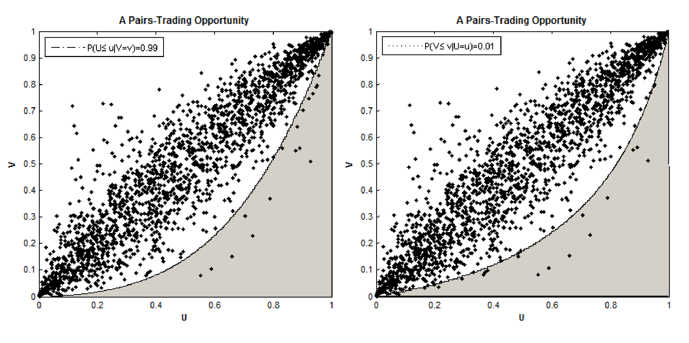
(Figure and Caption from Botha et al. 2013.) An illustration of the areas where the values of U and V respectively are considered extreme when using a 99% confidence level and the N14 copula dependence structure.

Conditional Probabilities

We start with a pair of stocks of interest \(S_1\) and \(S_2\), which can be selected by various methods. For example, using the Engle-Granger test for cointegration. By consensus, we define the spread as \(S_1\) in relation to \(S_2\). e.g. Short the spread means buying \(S_1\) and/or selling \(S_2\).

Use prices data of the stocks during the training/formation period, we proceed with a pseudo-MLE fit to establish a copula that reflects the relation of the two stocks during the training/formation period.

Then we can calculate the conditional probabilities using trading/testing period data:

\[\begin{split}\begin{align} P(U_1\le u_1 | U_2 = u_2), \\ P(U_2\le u_2 | U_1 = u_1). \end{align}\end{split}\]

• \(u_i \in [0, 1]\) is the quantile of trading period data mapped by a CDF formed in the training period.

• When \(P(U_1\le u_1 | U_2 = u_2) < 0.5\), then stock 1 is considered under-valued.

• When \(P(U_1\le u_1 | U_2 = u_2) > 0.5\), then stock 1 is considered over-valued.

Trading Logic

Now we define an upper threshold \(b_{up}\) (e.g. 0.95) and a lower threshold \(b_{lo}\) (e.g. 0.05), then the logic is as follows:

• If \(P(U_1\le u_1 | U_2 = u_2) \le b_{lo}\) and \(P(U_2\le u_2 | U_1 = u_1) \ge b_{up}\), then stock 1 is undervalued, and stock 2 is overvalued. Hence we long the spread. ( \(1\) in position)

• If \(P(U_2\le u_2 | U_1 = u_1) \le b_{lo}\) and \(P(U_1\le u_1 | U_2 = u_2) \ge b_{up}\), then stock 2 is undervalued, and stock 1 is overvalued. Hence we short the spread. ( \(-1\) in position)

• If both/either conditional probabilities cross the boundary of \(0.5\), then we exit the position, as we consider the position no longer valid. ( \(0\) in position)

Ambiguities and Comments

The authors did not specify what will happen if the followings occur:

1. When there is an open signal and an exit signal.

2. When there is an open signal and currently there is a position.

3. When there is a long and short signal together.

Here is our take:

1. Exit signal overrides open signal.

2. Flip the position to the signal’s suggestion. For example, originally have a short position, and receives a long signal, then the position becomes long.

3. Technically this should never happen with the default trading logic. However, if it did happen for whatever reason, long + short signal will lead to no opening signal and the positions will not change, unless there is an exit signal and that resets the position to 0.

For exiting a position, the authors proposed using ‘and’ logic: Both conditional probabilities need to cross \(0.5\). However, we found this too strict and sometimes fails to exit a position when it should. Therefore we also provide the ‘or’ logic: At least one of the conditional probabilities cross \(0.5\).

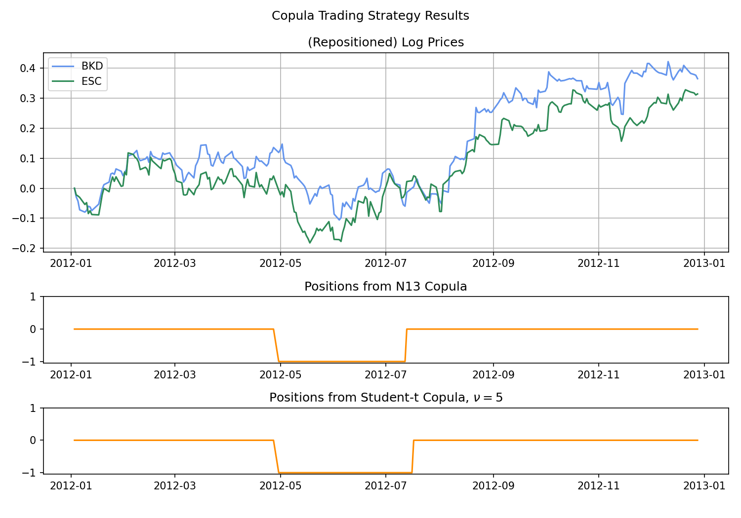
A visualised output of using a Student-t and N13 copula. The stock pair considered is BKD and ESC. The thresholds are 0.95 and 0.05.

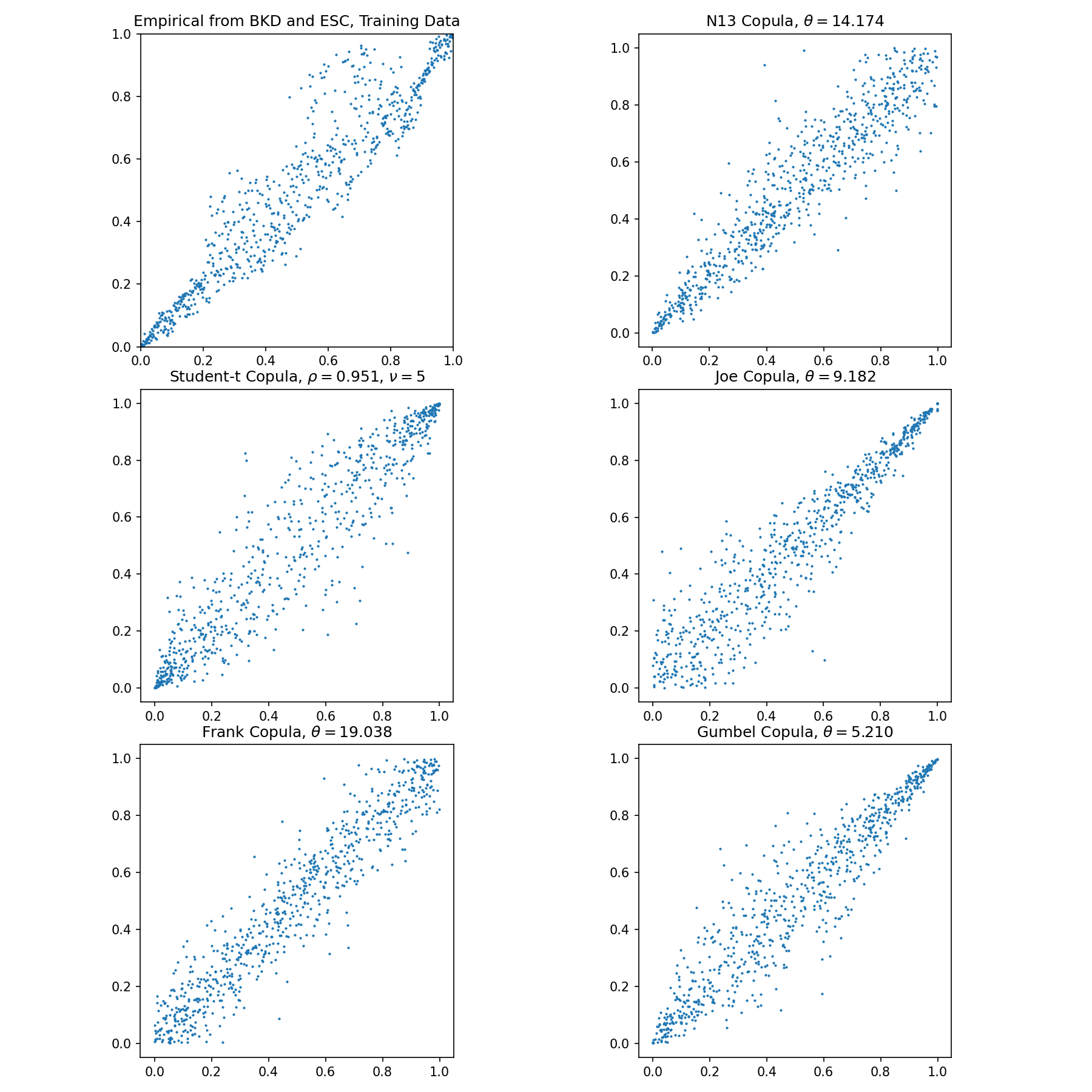
Sampling from the various fitted copulas, and plot the empirical density from training data from BKD and ESC.

Implementation

Note

The new BasicCopulaTradingRule class is created to allow on-the-go generation of trading signals and better management of opened and closed positions. It is a refactored version of the old BasicCopulaStrategy class that worked as a monolith, outputting trading signals for a pandas DataFrame. The new class takes price values one by one and generates signals to enter or exit the trade, making its integration into an existing trading pipeline easier.

Master module that implements the basic copula trading strategy.

This module is almost identical in terms of functionality as copula_strategy. But is designed with better efficiency, better structure, native pandas support, and supports mixed copulas. The trading logic is more clearly defined and all wrapped in one method for easier adjustment when needed, due to the ambiguities from the paper.

class BasicCopulaTradingRule(open_probabilities: Tuple[float, float] = (0.05, 0.95), exit_probabilities: Tuple[float, float] = (0.5, 0.5), exit_rule: str = 'and')

This module is a realization of the methodology in the following paper: Liew, R.Q. and Wu, Y., 2013. Pairs trading: A copula approach. Journal of Derivatives & Hedge Funds, 19(1), pp.12-30.

This is the threshold basic copula trading strategy implemented by [Liew et al. 2013]. First, one uses formation period prices to train a copula, then trade based on conditional probabilities calculated from the quantiles of the current price u1 and u2. If we define the spread as stock 1 in relation to stock 2, then the logic is as follows (All the thresholds can be customized via open_thresholds, exit_thresholds parameters):

• If P(U1 <= u1 | U2 = u2) <= 0.05 AND P(U2 <= u2 | U1 = u1) >= 0.95, then stock 1 is under-valued and stock 2 is over-valued. Thus we long the spread.

• If P(U1 <= u1 | U2 = u2) >= 0.95 AND P(U2 <= u2 | U1 = u1) <= 0.05, then stock 2 is under-valued and stock 1 is over-valued. Thus we short the spread.

• We close the position if the conditional probabilities cross with 0.5 (exit_probabilities).

For the exiting condition, the author proposed a closure when stock 1 AND 2’s conditional probabilities cross 0.5. However, we found it sometimes too strict and fails to exit a position when it should occasionally. Hence we also provide the OR logic implementation. You can use it by setting exit_rule=’or’. Also note that the signal generation is independent from the current position.

__init__(open_probabilities: Tuple[float, float] = (0.05, 0.95), exit_probabilities: Tuple[float, float] = (0.5, 0.5), exit_rule: str = 'and')

Class constructor.

Parameters:

• open_probabilities – (tuple) Optional. The default lower and upper threshold for opening a position for trading signal generation. Defaults to (0.05, 0.95).

• exit_probabilities – (tuple) Optional. The default lower and upper threshold for exiting a position for trading signal generation. Defaults to (0.5, 0.5).

• exit_rule – (str) Optional. The logic for triggering an exit signal. Available choices are ‘and’, ‘or’. They indicate whether both conditional probabilities need to cross 0.5. Defaults to ‘and’.

add_trade(start_timestamp: Timestamp, side_prediction: int, uuid: UUID | None = None)

Adds a new trade to track. Calculates trigger timestamp.

Parameters:

• start_timestamp – (pd.Timestamp) Timestamp of the future label.

• side_prediction – (int) External prediction for the future label.

• uuid – (str) Unique identifier used to link label to tradelog action.

check_entry_signal() → tuple

Function which checks entry condition based on self.current_probabilities.

• If P(U1 <= u1 | U2 = u2) <= 0.05 AND P(U2 <= u2 | U1 = u1) >= 0.95, then stock 1 is under-valued and stock 2 is over-valued. Thus we long the spread.

• If P(U1 <= u1 | U2 = u2) >= 0.95 AND P(U2 <= u2 | U1 = u1) <= 0.05, then stock 2 is under-valued and stock 1 is over-valued. Thus we short the spread.

Returns:

(tuple) Tuple of boolean entry flag and side (if entry flag is True).

set_cdf(cdf_x: Callable[[float], float], cdf_y: Callable[[float], float])

Set marginal C.D.Fs functions which transform X, Y values into probabilities, usually ECDFs are used. One can use construct_ecdf_lin function from copula_calculations module.

Parameters:

• cdf_x – (func) Marginal C.D.F. for series X.

• cdf_y – (func) Marginal C.D.F. for series Y.

set_copula(copula: object)

Set fit copula to self.copula.

Parameters:

copula – (object) Fit copula object.

update_probabilities(x_value: float, y_value: float)

Update latest probabilities (p1,p2) values from empirical x_value and y_value, where:

p1=self.copula.get_condi_prob(self.cdf_x(x_value), self.cdf_y(y_value)), p2=self.copula.get_condi_prob(self.cdf_y(y_value), self.cdf_x(x_value)),

As a result, updated probabilities are stored in self.current_probabilities and previous probabilities are stored in self.prev_probabilities. These containers are used to check entry/exit signals.

Parameters:

• x_value – (float) Latest value (price) for series X.

• y_value – (float) Latest value (price) for series Y.

update_trades(update_timestamp: Timestamp) → list

Checks whether any of the thresholds are triggered and currently open trades should be closed. Before using the method, one should have called self.update_probabilities() to update recent probalities.

Parameters:

update_timestamp – (pd.Timestamp) New timestamp to check vertical threshold.

Returns:

(list) List of closed trades.

Example

# Importing the module and other libraries
from arbitragelab.copula_approach import fit_copula_to_empirical_data
from arbitragelab.copula_approach.archimedean import Gumbel
from arbitragelab.trading.basic_copula import BasicCopulaTradingRule
import pandas as pd

# Instantiating the module with set open and exit probabilities
# and using the 'AND' exit logic:
cop_trading = BasicCopulaTradingRule(exit_rule='and', open_probabilities=(0.5, 0.95),
                                     exit_probabilities=(0.9, 0.5))

# Loading the data
pair_prices = pd.read_csv('PRICE_DATA.csv', index_col='Dates', parse_dates=True)

# Split data into train and test sets
prices_train = pair_prices.iloc[:int(len(s1_price)*0.7)]
prices_test = pair_prices.iloc[int(len(s1_price)*0.7):]

# Fitting copula to data and getting cdf for X and Y series
info_crit, fit_copula, ecdf_x, ecdf_y = fit_copula_to_empirical_data(x=prices_train['BKD'],
                                                                     y=prices_train['ESC'],
                                                                     copula=Gumbel)

# Printing fit scores (AIC, SIC, HQIC, log-likelihood)
print(info_crit)

# Setting initial probabilities
cop_trading.current_probabilities = (0.5, 0.5)
cop_trading.prev_probabilities = (0.5, 0.5)

# Adding copula to strategy
cop_trading.set_copula(fit_copula)

# Adding cdf for X and Y to strategy
cop_trading.set_cdf(cdf_x, cdf_y)

# Trading simulation
for time, values in prices_test.iterrows():
    x_price = values['BKD']
    y_price = values['ESC']

    # Adding price values
    cop_trading.update_probabilities(x_price, y_price)

    # Check if it's time to enter a trade
    trade, side = cop_trading.check_entry_signal()

    # Close previous trades if needed
    cop_trading.update_trades(update_timestamp=time)

    if trade:  # Open a new trade if needed
        cop_trading.add_trade(start_timestamp=time, side_prediction=side)

# Finally, check open trades at the end of the simulation
open_trades = cop_trading.open_trades

# And all trades that were opened and closed
closed_trades = cop_trading.closed_trades

Research Notebooks

The following research notebook can be used to better understand the copula strategy described above.

• Basic Copula Strategy

Download Notebook Download Sample Data

Research Article

Read our article on the topic

References

• Liew, R.Q. and Wu, Y., 2013. Pairs trading: A copula approach. Journal of Derivatives & Hedge Funds, 19(1), pp.12-30.

• Stander, Y., Marais, D. and Botha, I., 2013. Trading strategies with copulas. Journal of Economic and Financial Sciences, 6(1), pp.83-107.