Note

The following documentation closely follows the book by Ernest P. Chan: Algorithmic Trading: Winning Strategies and Their Rationale.

As well as the paper by Faik Bilgili: Stationarity and cointegration tests: Comparison of Engle-Granger and Johansen methodologies.

Tests for Cointegration

According to Ernest P. Chan: “The mathematical description of a mean-reverting price series is that the change of the price series in the next period is proportional to the difference between the mean price and the current price. This gives rise to the ADF test, which tests whether we can reject the null hypothesis that the proportionality constant is zero.”

The Augmented Dickey–Fuller (ADF) test is based on the idea that the current price level gives us information about the future price level: if it’s lower than the mean, the next move will be upwards, and vice versa.

The ADF test uses the linear model that describes the price changes as follows:

\[\Delta y(t) = \lambda y(t-1) + \mu + \beta t + \alpha_1 \Delta y(t-1) + ... + \alpha_k \Delta y(t-k) + \epsilon_t\]

where \(\Delta y(t) \equiv y(t) - y(t-1)\), \(\Delta y(t-1) \equiv y(t-1) - y(t-2)\), …

The hypothesis that is being tested is: \(\lambda = 0\). For simplicity we assume the drift term to be zero (\(\beta = 0\)). If we reject the hypothesis, this means that the next price move depends on the current price level.

Mean reversion tests, such as ADF usually require at least 90 percent certainty. But in practice, we can create strategies that are profitable even at lower certainty levels. The measure \(\lambda\) can be used to calculate the half-life, which indicates how long it takes for a price to mean revert:

\[\text{Half-life} = -log(2) / \lambda\]

Furthermore, we can see that if the \(\lambda\) value is positive, the price series are not mean-reverting. If it’s close to zero, the half-life is very long and the strategy won’t be profitable due to slow mean reversion.

Half-life period can be helpful to determine some of the parameters to use in the trading strategy. Say, if the half-life period is 20 days, then using 5 days backward-looking window for moving average or volatility calculation may not give the best results.

The most common approach is to use two cointegrated price series to construct a portfolio. This is done by simultaneously going long on one asset and short on the other, with an appropriate capital allocation for each asset. This approach is also called a “pairs trading strategy”. However, the approach can be extended to three and more assets.

Warning

From the mathematical standpoint, cointegration testing strives to prove that there exists at least one linear combination of given time series that is stationary. Hence sometimes during the testing, the cointegration vector might have only positive coefficients, making it not suitable for making a spread, while being completely theoretically sound.

Note

Another set of tools for pairs trading strategies is available in our Optimal Mean Reversion Module.

Johansen Cointegration Test

This is one of the most widely used cointegration tests, it’s upside is that it can be applied to multiple price series. Another common approach - the Cointegrated Augmented Dickey-Fuller (CADF) test can only be used on a pair of price series and is not covered in this module.

A motivation to use the Johansen approach instead of the simple ADF test is that, first it allows multiple price series for stationarity testing, and second it provides hedge ratios for price series used to combine elements into a stationary portfolio.

To understand how to test the cointegration of more than two variables, we can transform the equation used in the ADF test to a vector form. So \(y(t)\) would be vectors representing multiple price series, and the \(\lambda\) and \(\alpha\) are matrices. We also assume that the drift term is zero (\(\beta t = 0\)). So the equation can be rewritten as follows:

\[\Delta Y(t) = \Lambda Y(t-1) + M + A_1 \Delta Y(t-1) + ... + A_k \Delta Y(t-k) + \epsilon_t\]

This way we can test the hypothesis of \(\Lambda = 0\), in which case, we don’t have cointegration present. Denoting the rank of the obtained matrix \(\Lambda\) as \(r\) and the number of price series as \(n\), the number of independent portfolios that can be formed is equal to \(r\).

The Johansen test calculates the \(r\) and tests the hypotheses of \(r = 0\) (cointegrating relationship exists), \(r \le 1\), …, \(r \le n - 1\). In case all the above hypotheses are rejected, the result is that \(r = n\) and the eigenvectors of the \(\Lambda\) can be used as hedge ratios to construct a mean-reverting portfolio.

Note that the Johansen test is independent of the order of the price series, in contrast to the CADF test.

The Johansen test from the ArbitrageLab package allows getting the cointegration vectors, trace statistics, and eigenvector statistics from a given dataframe with price series. Note that the two last statistics will be calculated only if the input dataframe contains 12 or less price series.

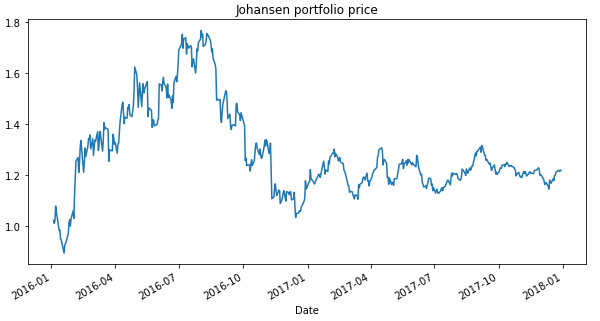
An example of a mean-reverting portfolio constructed using the Johansen test.

Implementation

This module implements the Johansen cointegration approach.

class JohansenPortfolio

The class implements the construction of a mean-reverting portfolio using eigenvectors from the Johansen cointegration test. It also checks Johansen (eigenvalue and trace statistic) tests for the presence of cointegration for a given set of assets.

__init__()

Class constructor.

construct_mean_reverting_portfolio(price_data: DataFrame, cointegration_vector: Series | None = None) → Series

When cointegration vector was formed, this function is used to multiply asset prices by cointegration vector to form mean-reverting portfolio which is analyzed for possible trade signals.

Parameters:

• price_data – (pd.DataFrame) Price data with columns containing asset prices.

• cointegration_vector – (pd.Series) Cointegration vector used to form a mean-reverting portfolio. If None, a cointegration vector with maximum eigenvalue from fit() method is used.

Returns:

(pd.Series) Cointegrated portfolio dollar value.

fit(price_data: DataFrame, dependent_variable: str | None = None, det_order: int = 0, n_lags: int = 1)

Finds cointegration vectors from the Johansen test used to form a mean-reverting portfolio.

Note: Johansen test yields several linear combinations that may yield mean-reverting portfolios. The function stores all of them in decreasing order of eigenvalue meaning that the first linear combination forms the most mean-reverting portfolio which is used in trading. However, researchers may use other stored cointegration vectors to check other portfolios.

This function will calculate and set johansen_trace_statistic and johansen_eigen_statistic only if the number of variables in the input dataframe is <=12. Otherwise it will generate a warning.

A more detailed description of this method can be found on p. 54-58 of “Algorithmic Trading: Winning Strategies and Their Rationale” by Ernie Chan.

This function is a wrapper around the coint_johansen function from the statsmodels.tsa module. Detailed descriptions of this function are available in the statsmodels documentation.

Parameters:

• price_data – (pd.DataFrame) Price data with columns containing asset prices.

• dependent_variable – (str) Column name which represents the dependent variable (y). By default, the first column is used as a dependent variable.

• det_order – (int) -1 for no deterministic term in Johansen test, 0 - for constant term, 1 - for linear trend.

• n_lags – (int) Number of lags used in the Johansen test. The practitioners use 1 as the default base value.

get_scaled_cointegration_vector(cointegration_vector: Series | None = None) → Series

This function returns the scaled values of the cointegration vector in terms of how many units of other cointegrated assets should be bought if we buy one unit of one asset.

Parameters:

cointegration_vector – (pd.Series) Cointegration vector used to form a mean-reverting portfolio. If None, a cointegration vector with maximum eigenvalue from fit() method is used.

Returns:

(pd.Series) The scaled cointegration vector values.

Examples

# Importing packages
import pandas as pd
from arbitragelab.cointegration_approach.johansen import JohansenPortfolio

# Getting the dataframe with time series of cointegrating asset prices
data = pd.read_csv('X_FILE_PATH.csv', index_col=0, parse_dates = [0])

# Running tests and finding test statistics and cointegration vectors
portfolio = JohansenPortfolio()
portfolio.fit(data)

# Getting results for the eigenvalue statistic test
eigenvalue_statistics = portfolio.johansen_trace_statistic

# Getting results for the trace statistic test
trace_statistics = portfolio.johansen_eigen_statistic

# Resulting cointegration vectors
cointegration_vectors = portfolio.cointegration_vectors

# Hedge ratios that can be used for spread construction
hedge_ratios = portfolio.hedge_ratios

Engle-Granger Cointegration Test

The cointegration testing approach proposed by Engle-Granger allows us to test whether two or more price series are cointegrated of a given order.

The Engle-Granger cointegration test is performed as follows:

• First, we need to determine the order of integration of variables \(x\) and \(y\) (or \(y_{1}, y_{2}, ...\) in case of more than two variables). If they are integrated of the same order, we can apply the cointegration test.

• Next, if the variables are integrated of order one at the previous step, the following regressions can be performed:

\[ \begin{align}\begin{aligned}x_t = a_0 + a_1 y_t + e_{1,t},\\y_t = b_0 + b_1 x_t + e_{2,t}\end{aligned}\end{align} \]

• Finally we run the following regressions and test for unit root for each equation:

\[ \begin{align}\begin{aligned}\Delta e_{1,t} = a_1 e_{1, t-1} + v_{1, t},\\\Delta e_{2,t} = a_2 e_{2, t-1} + v_{2, t}\end{aligned}\end{align} \]

If we cannot reject the null hypotheses that \(|a_1| = 0\) and \(|a_2| = 0\), we cannot reject the hypotheis that the variables are not cointegrated.

The hedge ratios for constructing a mean-reverting portfolio in the case of the Engle-Granger test are set to \(1\) for the \(x\) variable and the coefficient \(-a_1\) for the \(y\) variable (or \(-a_1, -a_2, ..\) in case of multiple \(y_i\) price series).

The Engle-Granger cointegration test implemented in the ArbitrageLab package assumes that the first step of the algorithm is passed and that the variables are integrated of order one. This test allows us to get cointegration vectors, ADF test statistics for the null hypotheses in the final step from a given dataframe with price series.

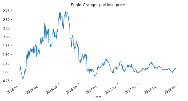
An example of a mean-reverting portfolio constructed using the Engle-Granger test.

Implementation

This module implements Engle-Granger cointegration approach.

class EngleGrangerPortfolio

The class implements the construction of a mean-reverting portfolio using the two-step Engle-Granger method. It also tests model residuals for unit-root (presence of cointegration).

__init__()

Class constructor method.

construct_mean_reverting_portfolio(price_data: DataFrame, cointegration_vector: Series | None = None) → Series

When cointegration vector was formed, this function is used to multiply asset prices by cointegration vector to form mean-reverting portfolio which is analyzed for possible trade signals.

Parameters:

• price_data – (pd.DataFrame) Price data with columns containing asset prices.

• cointegration_vector – (pd.Series) Cointegration vector used to form a mean-reverting portfolio. If None, a cointegration vector with maximum eigenvalue from fit() method is used.

Returns:

(pd.Series) Cointegrated portfolio dollar value.

fit(price_data: DataFrame, add_constant: bool = False)

Finds hedge-ratios using a two-step Engle-Granger method to form a mean-reverting portfolio. By default, the first column of price data is used as a dependent variable in OLS estimation.

This method was originally described in “Co-integration and Error Correction: Representation, Estimation, and Testing,” Econometrica, Econometric Society, vol. 55(2), pages 251-276, March 1987 by Engle, Robert F and Granger, Clive W J.

Parameters:

• price_data – (pd.DataFrame) Price data with columns containing asset prices.

• add_constant – (bool) A flag to add a constant term in linear regression.

static get_ols_hedge_ratio(price_data: DataFrame, dependent_variable: str, add_constant: bool = False) → Tuple[dict, DataFrame, Series, Series]

Get OLS hedge ratio: y = beta*X.

Parameters:

• price_data – (pd.DataFrame) Data Frame with security prices.

• dependent_variable – (str) Column name which represents the dependent variable (y).

• add_constant – (bool) Boolean flag to add constant in regression setting.

Returns:

(Tuple) Hedge ratios, X, and y and OLS fit residuals.

get_scaled_cointegration_vector(cointegration_vector: Series | None = None) → Series

This function returns the scaled values of the cointegration vector in terms of how many units of other cointegrated assets should be bought if we buy one unit of one asset.

Parameters:

cointegration_vector – (pd.Series) Cointegration vector used to form a mean-reverting portfolio. If None, a cointegration vector with maximum eigenvalue from fit() method is used.

Returns:

(pd.Series) The scaled cointegration vector values.

perform_eg_test(residuals: Series)

Perform Engle-Granger test on model residuals and generate test statistics and p values.

Parameters:

residuals – (pd.Series) OLS residuals.

Examples

# Importing packages
import pandas as pd
from arbitragelab.cointegration_approach.engle_granger import EngleGrangerPortfolio

# Getting the dataframe with time series of cointegrating asset prices
data = pd.read_csv('X_FILE_PATH.csv', index_col=0, parse_dates = [0])

# Running tests and finding test statistics and cointegration vectors
portfolio = EngleGrangerPortfolio()
portfolio.fit(data)

# Getting results for the ADF test in the last step of the method
adf_statistics = portfolio.adf_statistics

# Resulting cointegration vector
cointegration_vectors = portfolio.cointegration_vectors

# Hedge ratios that can be used for spread construction
hedge_ratios = portfolio.hedge_ratios

Research Notebooks

• Mean Reversion

Download Notebook Download Sample Data

Research Article

Read our article on the topic

Presentation Slides

References

• Chan, E., 2013. Algorithmic trading: winning strategies and their rationale (Vol. 625). John Wiley & Sons.

• Bilgili, F., 1998. Stationarity and cointegration tests: Comparison of Engle-Granger and Johansen methodologies.