Note

This document was greatly inspired by:

1. Nelsen, Roger B. An introduction to copulas. Springer Science & Business Media, 2007.

2. Nelsen, Roger B. “Properties and applications of copulas: A brief survey.” Proceedings of the first brazilian conference on statistical modeling in insurance and finance. University Press USP Sao Paulo, 2003.

3. Chang, Bo. Copula: A Very Short Introduction.

4. Andy Jones. SCAD penalty.

A Deeper Intro to Copulas

For people who are more interested in knowing more about copulas, where they come from, computation challenges, and the mathematical intuition behind it, this is the document to read. We advise the reader to go through A Practical Introduction to Copula at first for basic concepts that will be assumed in this document.

Definition (Formal definition of bivariate copula) A two-dimensional copula is a function \(C: \mathbf{I}^2 \rightarrow \mathbf{I}\) where \(\mathbf{I} = [0, 1]\) such that

• (C1) \(C(0, x) = C(x, 0) = 0\) and \(C(1, x) = C(x, 1) = x\) for all \(x \in \mathbf{I}\);

• (C2) \(C\) is 2-increasing, i.e., for \(a, b, c, d \in \mathbf{I}\) with \(a \le b\) and \(c \le d\):

  \[V_c \left( [a,b]\times[c,d] \right) := C(b, d) - C(a, d) - C(b, c) + C(a, c) \ge 0.\]

Keep in mind that the definition of copula \(C\) is just the joint cumulative density on quantiles of each marginal random variable (r.v.). i.e.,

\[C(u_1, u_2) = \mathbb{P}(U_1 \le u_1, U_2 \le u_2).\]

And (C1)(C2) naturally comes from joint CDF: (C1) is quite obvious, and (C2) is just the definition of

\[\mathbb{P}(a \le U_1 \le b, c \le U_2 \le d).\]

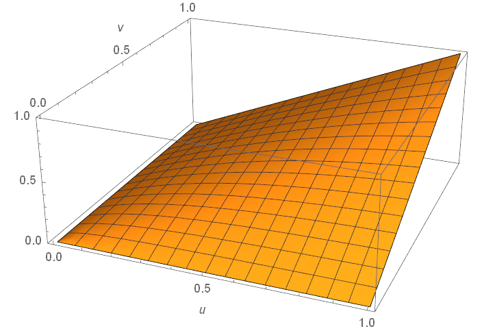
Plot of \(C(u,v)\) for an N13 copula.

A Few Useful Things

Before we begin, let us make it clear that this documentation is not meant to be purely theoretical, and we are treating copulas from an applied probability theory point of view with a focus on trading. To achieve this, we need to introduce a few useful concepts that will for sure help. To avoid getting lost in symbols, we only discuss bivariate copulas here.

Tail Dependence

Definition (Coefficients of lower and upper tail dependence) The lower and upper tail dependence are defined respectively as:

\[\lambda_l := \lim_{q \rightarrow 0^+} \mathbb{P}(U_2 \le q \mid U_1 \le q),\]

\[\lambda_u := \lim_{q \rightarrow 1^-} \mathbb{P}(U_2 > q \mid U_1 > q).\]

And those can be derived from the copula:

\[\lambda_l = \lim_{q \rightarrow 0^+} \frac{\mathbb{P}(U_2 \le q, U_1 \le q)}{\mathbb{P}(U_1 \le q)} = \lim_{q \rightarrow 0^+} \frac{C(q,q)}{q},\]

\[\lambda_u = \lim_{q \rightarrow 1^-} \frac{\mathbb{P}(U_2 > q, U_1 > q)}{\mathbb{P}(U_1 > q)} = \lim_{q \rightarrow 1^-} \frac{\hat{C}(q,q)}{q},\]

where \(\hat{C}(u_1, u_2) = u_1 + u_2 - 1 + C(1 - u_1, 1 - u_2)\) is the reflected copula. If \(\lambda_l > 0\) then there is lower tail dependence. If \(\lambda_u > 0\) then there is upper tail dependence. Note that one should actually calculate the limit for each copula, and it is not obvious from the plot usually.

For example, as plotted below, it can be calculated easily that for a Gumbel copula, \(\lambda_l=0\) and \(\lambda_u=1\).

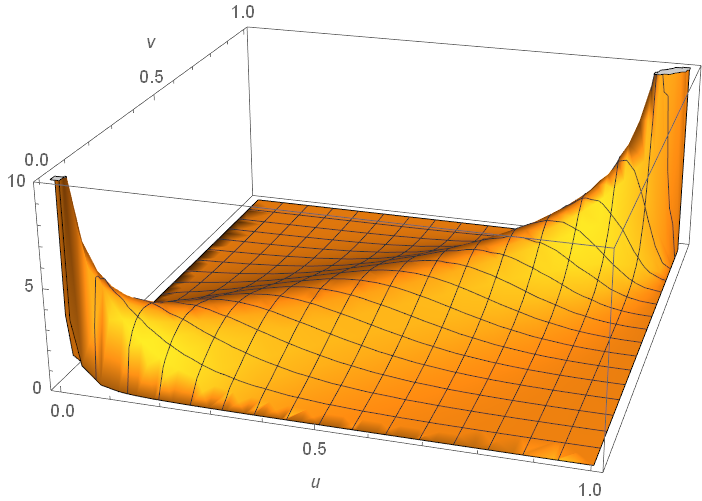
Plot of \(c(u,v)\) for a Gumbel copula. It has upper tail dependence but no lower tail dependence.

Fréchet–Hoeffding Bounds

Here is a handy theorem that holds true for all copulas, and is quite useful in analysis:

Theorem (Fréchet–Hoeffding Bounds for bivariate copulas) Consider a bivariate copula \(C(u_1, u_2)\), then for \(u_j \in \mathbf{I}\):

\[\max \{ u_1 + u_2 - 1 \} \le C(u_1, u_2) \le \min\{u_1, u_2\}.\]

The lower bound comes from the counter-monotonicity copulas whereas the upper bound comes from the co-monotonicity copulas. co-monotone means the two marginal random variables are perfectly positively dependent, for instance, \(X_2 = 3 X_1\). In this case their quantiles are identical and we have:

\[\begin{split}\begin{align} C(u_1, u_2) &= \mathbb{P}(U_1 \le u_1, U_2 \le u_2) \\ &= \mathbb{P}(U_1 \le u_1, U_1 \le u_2) \\ &= \mathbb{P}(U_1 \le \min\{u_1, u_2\}). \end{align}\end{split}\]

Similarly, counter-monotone means the two random variables are perfectly negatively dependent, for instance, \(X_2 = -5 X_1\).

Empirical Copula

At first, a copula always exists for two continuous random variables (to avoid ties in percentile) \(X_1\), \(X_2\), guaranteed by Sklar’s theorem. Once we have enough observations from \(X_1\) and \(X_2\), we define the implied bivariate empirical copula as follows:

\[\tilde{C}_n(\frac{i}{n}, \frac{j}{n}) = \frac{1}{n} ||\{ (X_1, X_2) \mid X_1 \le X_1(i), X_2 \le X_2(j) \}||,\]

where \(X_1(i)\) is the \(i\)-th largest element for \(X_1\); same applies for \(X_2(j)\); \(|| \cdot ||\) is the cardinality, or the number of elements in the set for a finite set. The definition may look more complicated than what it is. To calculate \(\tilde{C}_n(\frac{i}{n}, \frac{j}{n})\), one just need to count the number of cases in the whole observation that are not greater than the \(i\)-th and \(j\)-th rank for their own marginal r.v. respectively.

The empirical copula can also be defined parametrically by finding each margincal CDF \(F_1\), \(F_2\). In that case, the empirical copula becomes:

\[\tilde{C}_n(u_1, u_2) = \frac{1}{n} ||\{ (X_1, X_2) \mid F_1^{-1}(X_1) \le u_1, F_2^{-1}(X_2) \le u_2 \}||,\]

If one uses empirical CDFs, then it is identical to our first definition.

Note

Implicitly, copula is used to model independent draws from multiple time-invariant r.v.’s and analyze their dependency structure without influence from the specific marginal distributions. When applying copula to time series, obviously each draw is not independent, and the dependency between securities is likely to change as time progresses. Therefore, using an empirical copula may not be a good idea.

Also, using a non-parametric empirical copula for trading may “downscale” the strategy into its simpler counterparts that one may aim to improve upon in the beginning. For example, since most copula-based trading strategies uses conditional probabilities to signal thresholds. If one directly uses an empirical copula, then it technically becomes a rank-based distance method: Simply look at the history and see how unlikely such mispricing events happens. If they are really mispriced based on ranks then open a position. This rather common strategy may already be overused and not generate enough alpha. Plus, one will lose the ability to carefully model the tail dependencies at their own desire.

“Pure” Copulas

Note

“Pure” copula is not an official name. It is used here for convenience, in contrast to mixed copulas, to represent Archimedean and elliptical copulas.

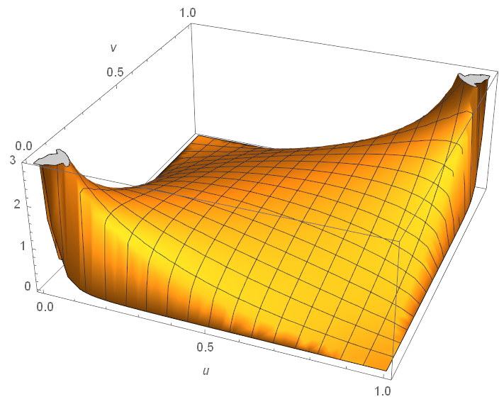
Plot of \(c(u,v)\) for the infamous Gaussian copula. It is often not obvious to decide from the plot that whether a copula has tail dependencies.

For practical purposes, at least for the implemented trading strategies in this module, it is enough to understand tail dependency for each copula and what structure are they generally modeling, because sometimes the nuances only come into play for a (math) analyst. Here are a few key results:

1. Upper tail dependency means the two random variables are likely to have large values together. For instance, when working with returns series, upper tail dependency implies that the two stocks are likely to have large gains together.

2. Lower tail dependency means the two random variables are likely to have small values together. This is much stronger in general compared to upper tail dependency, because stocks are more likely to go down together than going up together.

3. Frank and Gaussian copulas do not have tail dependencies at all. And Gaussian copula infamously contributed to the 2008 financial crisis by pricing CDOs exactly for this reason. Frank copula has a stronger dependence in the center compared to Gaussian.

4. For fitting prices and returns data, usually Student-t comes top score. Also it does not give probabilities far away from an empirical copula.

5. For Value-at-Risk calculations, Gaussian copula is overly optimistic and Gumbel is too pessimistic.

6. Copulas with upper tail dependency: Gumbel, Joe, N13, N14, Student-t.

7. Copulas with lower tail dependency: Clayton, N14 (weaker), Student-t.

8. Copulas with no tail dependency: Gaussian, Frank.

Since a Student-t copula will converge to a Gaussian copula as the degrees of freedom increases, it makes sense to quantify the change of tail dependence (the upper and lower tail dependency is the same value thanks to symmetry for Student-t copula). It is tabled below from [Demarta, McNeil, The t Copula and Related Copulas, 2005]:

Tail Dependency for Bivariate Student-t Copula

\(\nu \downarrow, \rho \rightarrow\)	-0.5	0	0.5	0.9	1
2	0.06	0.18	0.39	0.72	1
4	0.01	0.08	0.25	0.63	1
10	0	0.01	0.08	0.46	1
\(\infty\)	0	0	0	0	1

Creating own copulas

A user can create one of Archimedean or elliptical copula object and play around with it.

Archimedean copulas

Note

All copula classes in this module share the same basic public methods.

Here we only demonstrate all methods for the Gumbel copula class, as an example. All other classes have the same methods available

This module implements Archimedean Copulas.

class Gumbel(theta: float | None = None, threshold: float = 1e-10)

Gumbel Copula.

__init__(theta: float | None = None, threshold: float = 1e-10)

Initiate a Gumbel copula object.

Parameters:

• theta – (float) Range in [1, +inf), measurement of copula dependency.

• threshold – (float) Optional. Below this threshold, a percentile will be rounded to the threshold.

describe() → Series

Print the description of the copula’s name and parameter as a pd.Series.

Note: the descriptive name is different from the copula’s class name, but its full actual name. E.g. The Student copula class has its descriptive name as ‘Bivariate Student-t Copula’.

Return description:

(pd.Series) The description of the copula, including its descriptive name, class name, and its parameter(s) when applicable.

fit(u: array, v: array) → float

Fit copula to empirical data (pseudo-observations). Once fit, self.theta is updated.

Parameters:

• u – (np.array) 1D vector data of X pseudo-observations. Need to be uniformly distributed [0, 1].

• v – (np.array) 1D vector data of Y pseudo-observations. Need to be uniformly distributed [0, 1].

Returns:

(float) Theta hat estimate for fit copula.

get_condi_prob(u: float, v: float, eps: float = 1e-05) → float

Calculate conditional probability function: P(U<=u | V=v).

Result is analytical. Also the u and v will be remapped into [eps, 1-eps] to avoid edge values that may result in infinity or NaN.

Note: This probability is symmetric about (u, v).

Parameters:

• u – (float) A real number in [0, 1].

• v – (float) A real number in [0, 1].

• eps – (float) Optional. The distance to the boundary 0 or 1, such that the value u, v will be mapped back. Defaults to 1e-5.

Returns:

(float) The conditional probability.

get_cop_density(u: float, v: float, eps: float = 1e-05) → float

Get the copula density c(u, v).

Result is analytical. Also the u and v will be remapped into [eps, 1-eps] to avoid edge values that may result in infinity or NaN.

Parameters:

• u – (float) A real number in [0, 1].

• v – (float) A real number in [0, 1].

• eps – (float) Optional. The distance to the boundary 0 or 1, such that the value u, v will be mapped back. Defaults to 1e-5.

Returns:

(float) The probability density (aka copula density).

get_cop_eval(u: float, v: float, eps: float = 1e-05) → float

Get the evaluation of copula, equivalently the cumulative joint distribution C(u, v).

Result is analytical. Also the u and v will be remapped into [eps, 1-eps] to avoid edge values that may result in infinity or NaN.

Parameters:

• u – (float) A real number in [0, 1].

• v – (float) A real number in [0, 1].

• eps – (float) Optional. The distance to the boundary 0 or 1, such that the value u, v will be mapped back. Defaults to 1e-5.

Returns:

(float) The evaluation of copula (aka cumulative joint distribution).

get_log_likelihood_sum(u: array, v: array) → float

Get log-likelihood value sum.

Parameters:

• u – (np.array) 1D vector data of X pseudo-observations. Need to be uniformly distributed [0, 1].

• v – (np.array) 1D vector data of Y pseudo-observations. Need to be uniformly distributed [0, 1].

Returns:

(float) Log-likelihood sum value.

plot_cdf(plot_type: str = '3d', grid_size: int = 50, levels: list | None = None, **kwargs) → axis

Plot either ‘3d’ or ‘contour’ plot of copula CDF.

Parameters:

• plot_type – (str) Either ‘3d’ or ‘contour’(2D) plot.

• grid_size – (int) Mesh grid granularity.

• kwargs – (dict) User-specified params for ‘ax.plot_surface’/’plt.contour’.

• levels – (list) List of float values that determine the number and levels of lines in a contour plot. If not provided, these are calculated automatically.

Returns:

(plt.axis) Axis object.

plot_pdf(plot_type: str = '3d', grid_size: int = 50, levels: list | None = None, **kwargs) → Figure

Plot either ‘3d’ or ‘contour’ plot of copula PDF.

Parameters:

• plot_type – (str) Either ‘3d’ or ‘contour’(2D) plot.

• grid_size – (int) Mesh grid granularity.

• levels – (list) List of float values that determine the number and levels of lines in a contour plot. If not provided, these are calculated automatically.

Returns:

(plt.axis) Axis object.

plot_scatter(num_points: int = 100) → Axes

Plot copula scatter plot of generated pseudo-observations.

Parameters:

num_points – (int) Number of samples to generate.

Returns:

(plt.axis) Axis object.

sample(num: int | None = None, unif_vec: array | None = None) → array

Generate pairs according to P.D.F., stored in a 2D np.array.

User may choose to side-load independent uniformly distributed data in [0, 1].

Parameters:

• num – (int) Number of points to generate.

• unif_vec – (np.array) Shape=(num, 2) array, two independent uniformly distributed sets of data. Default uses numpy pseudo-random generators.

Returns:

(np.array) Shape=(num, 2) array, sampled data for this copula.

static theta_hat(tau: float) → float

Calculate theta hat from Kendall’s tau from sample data.

Parameters:

tau – (float) Kendall’s tau from sample data.

Returns:

(float) The associated theta hat for this very copula.

class Clayton(theta: float | None = None, threshold: float = 1e-10)

Clayton copula.

__init__(theta: float | None = None, threshold: float = 1e-10)

Initiate a Clayton copula object.

Parameters:

• theta – (float) Range in [-1, +inf) {0}, measurement of copula dependency.

• threshold – (float) Optional. Below this threshold, a percentile will be rounded to the threshold.

class Joe(theta: float | None = None, threshold: float = 1e-10)

Joe Copula.

__init__(theta: float | None = None, threshold: float = 1e-10)

Initiate a Joe copula object.

Parameters:

• theta – (float) Range in [1, +inf), measurement of copula dependency.

• threshold – (float) Optional. Below this threshold, a percentile will be rounded to the threshold.

class Frank(theta: float | None = None, threshold: float = 1e-10)

Frank Copula.

__init__(theta: float | None = None, threshold: float = 1e-10)

Initiate a Frank copula object.

Parameters:

• theta – (float) All reals except for 0, measurement of copula dependency.

• threshold – (float) Optional. Below this threshold, a percentile will be rounded to the threshold.

class N13(theta: float | None = None, threshold: float = 1e-10)

N13 Copula (Nelsen 13).

__init__(theta: float | None = None, threshold: float = 1e-10)

Initiate an N13 copula object.

Parameters:

• theta – (float) Range in [0, +inf), measurement of copula dependency.

• threshold – (float) Optional. Below this threshold, a percentile will be rounded to the threshold.

class N14(theta: float | None = None, threshold: float = 1e-10)

N14 Copula (Nelsen 14).

__init__(theta: float | None = None, threshold: float = 1e-10)

Initiate an N14 copula object.

Parameters:

• theta – (float) Range in [1, +inf), measurement of copula dependency.

• threshold – (float) Optional. Below this threshold, a percentile will be rounded to the threshold.

Elliptical copulas

Note

Elliptical copulas (Gaussian and T-Student copulas) can also work in N-dimensional space, however current implementations only support a 2-dimensional case. Multi-dimensional elliptical copulas will be added in future updates of ArbitrageLab.

This module implements Elliptical Copulas.

class GaussianCopula(cov: array | None = None)

Bivariate Gaussian Copula.

__init__(cov: array | None = None)

Initiate a Gaussian copula object.

Parameters:

cov – (np.array) Covariance matrix (NOT correlation matrix), measurement of covariance. The class will calculate correlation internally once the covariance matrix is given.

Note

For Student copula, there is a special function used to find optimal \(\nu\) parameter for Student distribution used in Student Copula.

fit_nu_for_t_copula(u: array, v: array, nu_tol: float | None = None) → float

Find the best fit value nu for Student-t copula.

This method finds the best value of nu for a Student-t copula by maximum likelihood, using COBYLA method from scipy.optimize.minimize. nu’s fit range is [1, 15]. When the user wishes to use nu > 15, please delegate to Gaussian copula instead. This step is relatively slow.

Parameters:

• u – (np.array) 1D vector data of X pseudo-observations. Need to be uniformly distributed [0, 1].

• v – (np.array) 1D vector data of Y pseudo-observations. Need to be uniformly distributed [0, 1].

• nu_tol – (float) The final accuracy for finding nu.

Returns:

(float) The best fit of nu by maximum likelihood.

class StudentCopula(nu: float | None = None, cov: array | None = None)

Bivariate Student-t Copula, need degree of freedom nu.

__init__(nu: float | None = None, cov: array | None = None)

Initiate a Student copula object.

Parameters:

• nu – (float) Degrees of freedom.

• cov – (np.array) Covariance matrix (NOT correlation matrix), measurement of covariance. The class will calculate correlation internally once the covariance matrix is given.

Examples

# Importing the functionality
from arbitragelab.copula_approach.archimedean import Gumbel
from arbitragelab.copula_approach.elliptical import StudentCopula, fit_nu_for_t_copula

cop = Gumbel(theta=2)
# Check copula description
descr = cop.describe()

# Get cdf, pdf, conditional cdf
cdf = cop.get_cop_density(0.5, 0.7)
pdf = cop.get_cop_eval(0.5, 0.7)
cond_cdf = cop.get_condi_prob(0.5, 0.7)

# Sample from copula
sample = cop.sample(num=100)

# Fit copula to some data
cop.fit([0.5, 0.2, 0.3, 0.2, 0.1, 0.99],
        [0.1, 0.02, 0.9, 0.22, 0.11, 0.79])
print(cop.theta)

# Generate copula plots
cop.plot_scatter(200)
cop.plot_pdf('3d')
cop.plot_pdf('contour')
cop.plot_cdf('3d')
cop.plot_cdf('contour')

# Creating Student copula
nu = fit_nu_for_t_copula([0.5, 0.2, 0.3, 0.2, 0.1, 0.99],
                         [0.1, 0.02, 0.9, 0.22, 0.11, 0.79])
student_cop = StudentCopula(nu=nu, cov=None)
student_cop.fit([0.5, 0.2, 0.3, 0.2, 0.1, 0.99],
                [0.1, 0.02, 0.9, 0.22, 0.11, 0.79])

Applying copula to empirical data

As it was previously discussed, in order to use copula, one first needs to fit it on empirical data and find its corresponding parameter - theta for Archimedean copulas and rho/cov for elliptical.

However, copulas take only pseudo-observations distributed in \([0, 1]\). One can either use statsmodels.distributions.empirical_distribution.ECDF or ArbitrageLab’s function construct_ecdf_lin which is a slight modification of statsmodels’ ECDF with linear interpolation between data points.

construct_ecdf_lin(train_data: array, upper_bound: float = 0.99999, lower_bound: float = 1e-05) → Callable

Construct an empirical cumulative density function with linear interpolation between data points.

The function it returns agrees with the ECDF function from statsmodels in values, but also applies linear interpolation to fill the gap. Features include: Allowing training data to have nan values; Allowing the cumulative density output to have an upper and lower bound, to avoid singularities in some applications with probability 0 or 1.

Parameters:

• train_data – (np.array) The data to train the output ecdf function.

• upper_bound – (float) The upper bound value for the returned ecdf function.

• lower_bound – (float) The lower bound value for the returned ecdf function.

Returns:

(Callable) The constructed ecdf function.

However, one can fit several copulas to the same dataset. The question is: “Which copula suits best for the empirical data?”

Usually, one can either use:

1. Akaike Information Criterion (AIC).

2. Schwarz information criterion (SIC).

3. Hannan-Quinn information criterion(HQIC).

All of the information criteria use log_likelihood from get_log_likelihood_sum function for estimation. The best copula is the one that yields the minimum AIC, SIC or HQIC value.

aic(log_likelihood: float, n: int, k: int = 1) → float

Akaike information criterion.

Parameters:

• log_likelihood – (float) Sum of log-likelihood of some data.

• n – (int) Number of instances.

• k – (int) Number of parameters estimated by max likelihood.

Returns:

(float) Value of AIC.

sic(log_likelihood: float, n: int, k: int = 1) → float

Schwarz information criterion (SIC), aka Bayesian information criterion (BIC).

Parameters:

• log_likelihood – (float) Sum of log-likelihood of some data.

• n – (int) Number of instances.

• k – (int) Number of parameters estimated by max likelihood.

Returns:

(float) Value of SIC.

hqic(log_likelihood: float, n: int, k: int = 1) → float

Hannan-Quinn information criterion.

Parameters:

• log_likelihood – (float) Sum of log-likelihood of some data.

• n – (int) Number of instances.

• k – (int) Number of parameters estimated by max likelihood.

Returns:

(float) Value of HQIC.

On the other hand, one can just use the ArbitrageLab function which takes empirical data -> gets ECDFs -> fits copula, and returns fit copula object. It also returns fit ECDF(x), ECDF(y) functions, and information criterion values which can be used to find the best copula for the current dataset.

fit_copula_to_empirical_data(x: array, y: array, copula: Copula) → tuple

Fit copula to empirical data and generate goodness-of-fit statistics as well as empirical CDFs used in estimation.

If fitting a Student-t copula, it also includes a max likelihood fit for nu using COBYLA method from scipy.optimize.minimize. nu’s fit range is [1, 15]. When the user wishes to use nu > 15, please delegate to Gaussian copula instead. This step is relatively slow.

The output returns:

• result_dict: (dict) The name of the copula and its SIC, AIC, HQIC values;

• copula: (Copula) The fitted copula with parameters satisfying maximum likelihood;

• s1_cdf: (func) The cumulative density function for stock 1, using training data;

• s2_cdf: (func) The cumulative density function for stock 2, using training data.

Parameters:

• x – (np.array) 1D stock time series data in desired form.

• y – (np.array) 1D stock time series data in desired form.

• copula – (Copula) Copula class to fit.

Returns:

(dict, Copula, func, func) The name of the copula and its SIC, AIC, HQIC values; The fitted copula with parameters satisfying maximum likelihood; The cumulative density function for series 1, using training data; The cumulative density function for series 2, using training data.

Examples

# Importing the functionality
import pandas as pd
from arbitragelab.copula_approach import fit_copula_to_empirical_data
from arbitragelab.copula_approach.archimedean import (Gumbel, Clayton, Frank,
                                                      Joe, N13, N14)
from arbitragelab.copula_approach.elliptical import (StudentCopula,
                                                     GaussianCopula)

# Importing data
bkd_prices = pd.read_csv('BKD.csv', index_col=0)
esc_prices = pd.read_csv('ECS.csv', index_col=0)

bkd_returns = bkd_prices.pct_change().dropna()
esc_returns = esc_prices.pct_change().dropna()

# All Archimedean and Elliptical copulas to fit
copulas = [Gumbel, Clayton, Frank, Joe, N13, N14, GaussianCopula, StudentCopula]
aics = dict()

for cop in copulas:
    info_crit_logs, fit_copula, ecdf_x, ecdf_y = fit_copula_to_empirical_data(x=bkd_prices,
                                                                              y=esc_returns,
                                                                              copula=cop)
    aics[info_crit_logs['Copula Name']] = info_crit_logs['AIC']

# AIC values for all copulas
print(aics)

Mixed Copulas

In this copula_approach module, we support two mixed copula classes: CFGMixCop for Clayton-Frank-Gumbel mix and CTGMixCop for Clayton-Student-Gumbel mix, inspired by [da Silva et al. 2017].

It is pretty intuitive to understand, for example, for a CFG mixed copula, one needs to specify the \(\theta\)’s, the dependency parameter for each copula component, and their weights that sum to \(1\). In total there are \(5\) parameters for CFG. The weights should be understood in the sense of Markov, i.e., it describes the probability of an observation coming from each component.

For example, we present the Clayton-Frank-Gumbel mixed copula as below:

\[C_{mix}(u_1, u_2; \boldsymbol{\theta}, \mathbf{w}) := w_C C_C(u_1, u_2; \theta_C) + w_F C_F(u_1, u_2; \theta_F) + w_G C_G(u_1, u_2; \theta_G)\]

Why Mixed Copulas

Archimedean copulas and elliptical copulas, though powerful by themselves to capture nonlinear relations for two random variables, may suffer from the degree to which they can be calibrated to data. While using a pure empirical copula may subject to overfiting, a mixed copula that can calibrate the upper and lower tail dependency usually describes the dependency structure really well for its flexibility.

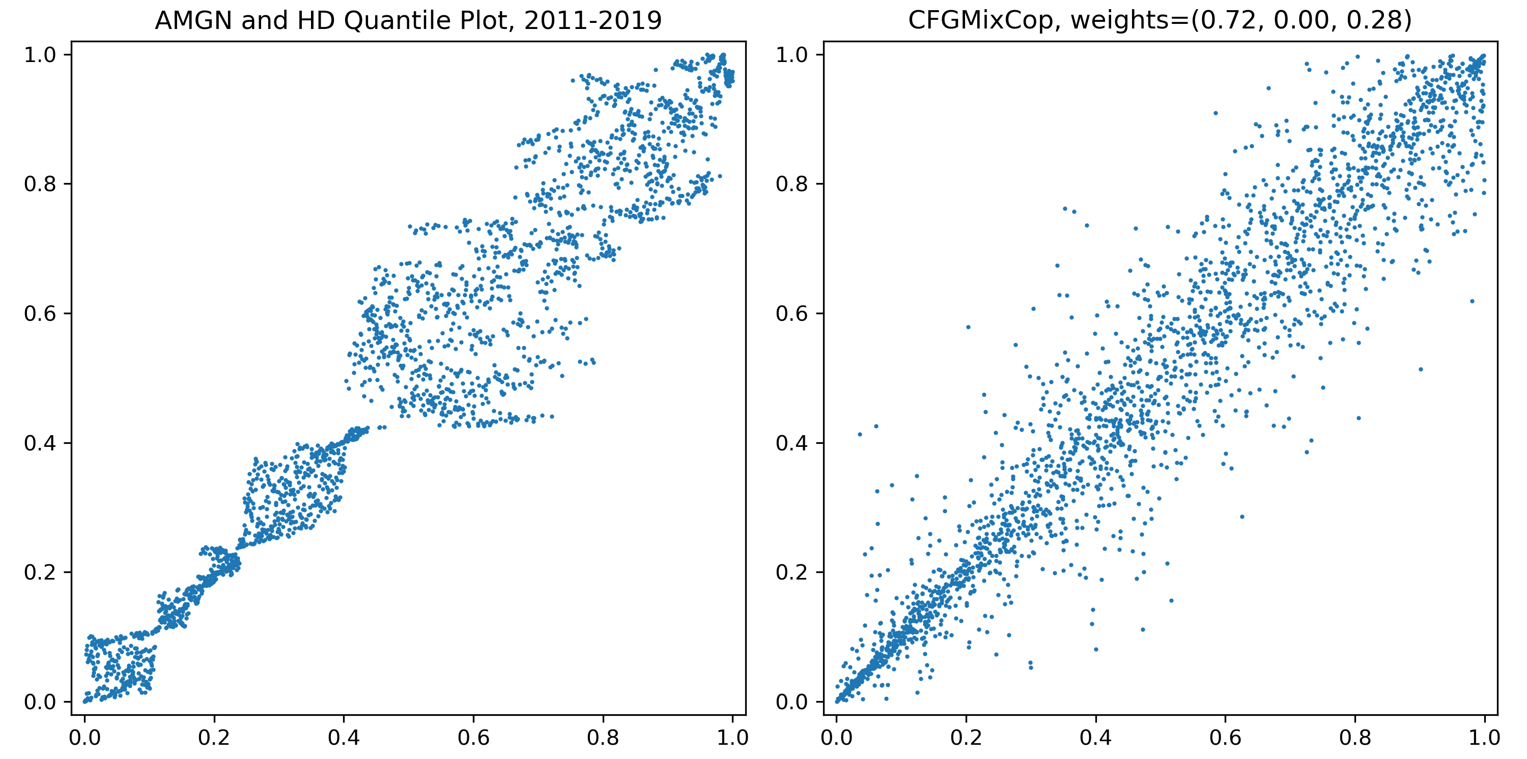
Plot of quantiles for prices of Amgen and Home Depot in 2011-2019, and sample plots from a fitted CFG copula. Mixed copulas calibrate the tail dependencies better than “pure” copulas.

But this flexibility comes at a price: fitting it to data is not trivial. Although one can wrap an optimization function for finding the individual weights and copula parameters using max likelihood, realistically this is a bad practice for the following reasons:

1. The outcome is highly unstable, and is heavily subject to the choice of the maximization algorithm.

2. A maximization algorithm fitting \(5\) parameters for CFG or \(6\) parameters for CTG usually tends to settle to a bad result that does not yield a comparable advantage to even its component copula. For example, sometimes the fit score for CTG is worse than a direct pseudo-max likelihood fit for Student-t copula.

3. Sometimes there is no result for the fit, since the algorithm does not converge.

4. Some maximization algorithms use Jacobian or Hessian matrix, and for some copulas the derivative computation is not numerically stable.

5. Often the weight of a copula component is way too small to be reasonable. For example, when an algorithm says there is \(0.1 \%\) Gumbel copula weight in a dataset of \(1000\) observations, then there is on average \(1\) observation that comes from Gumbel copula. It is bad modeling in every sense.

EM Fitting Algorithm

Instead, we adopt a two-step expectation-maximization (EM) algorithm for fitting mixed copulas, adapted from [Cai, Wang 2014]. This algorithm addresses all the above disadvantages of a generic maximization optimizer. The only downside is that, the CTG copula may take a while to converge to a solution for certain data sets.

Suppose we are working on a three-component mixed copula of bivariate Archimedeans and ellipticals. We aim to maximize over the objective function for copula parameters \(\boldsymbol{\theta}\) and weights \(\mathbf{w}\).

\[Q(\boldsymbol{\theta}, \mathbf{w}) = \sum_{t=1}^T \log \left[ \sum_{k=1}^3 w_k c_k(u_{1,t}, u_{2,t}; \theta_k) \right] - T \sum_{k=1}^3 p_{\gamma, a}(w_k) + \delta \left( \sum_{k=1}^s w_k - 1 \right),\]

where \(T\) is the length of the training set, or the size of the observations; \(k\) is the dummy variable for each copula component; \(p_{\gamma, a}(\cdot)\) is the smoothly clipped absolute deviation (SCAD) penalty term with tuning parameters \(\gamma`and :math:`a\) and it is the term that drives small copula components to \(0\); and last but not least \(\delta\) the Lagrange multiplier term that will be used for the E-step is:

\[\delta = T p'_{\gamma, a}(w_k) - \sum_{t=1}^T \frac{c_k(u_{1,t}, u_{2,t}; \theta_k)} {\sum_{j=1}^3 w_{j} c_{j}(u_{1,t}, u_{2,t}; \theta_{j})}\]

E-step

Iteratively calculate the following using the old \(\boldsymbol{\theta}\) and \(\mathbf{w}\) until it converges:

\[w_k^{new} = \left[ w_k p'_{\gamma, a}(w_k) - \frac{1}{T} \sum_{t=1}^T \frac{c_k(u_{1,t}, u_{2,t}; \theta_k)} {\sum_{j=1}^3 w_{j} c_{j}(u_{1,t}, u_{2,t}; \theta_{j})} \right] \times \left[ \sum_{j=1}^3 w_{j} p'_{\gamma, a}(w_{j}) \right]^{-1}\]

M-step

Use the updated weights to find new \(\boldsymbol{\theta}\), such that \(Q\) is maximized. One can use truncated Newton or Newton-Raphson for this step. This step, though still a wrapper around some optimization function, is much better than estimating the weights and copula parameters all together.

We then iterate the two steps until it converges. It is tested that the EM algorithm is oracle and sparse. Loosely speaking, the former means it has good asymptotic properties, and the latter says it will trim small weights off.

Note

The EM algorithm is still not mathematically perfect, and has the following issues:

1. It is slow for some data sets. Also the CTG is slow due to the bottleneck from Student-t copula.

2. If the copulas mixture have similar components, for instance, Gaussian and Frank, then it cannot pick the correct component weights well. Luckily for fitting data, usually the differences are minimal.

3. The SCAD parameters \(\gamma\) and \(a\) may require some tuning, depending on the data set it fits. Some authors suggest using cross validation to find a good pair of values. We did not implement this in the package because it takes really long for the calculation to a point it becomes unrealistic to run it (about 1 hour in some cases). We did run some CV while coding it, so that the default values of \(\gamma\) and \(a\) are good choices.

4. Sometimes the algorithm throws warnings, because the optimization algorithm underneath does not strictly follow the prescribed bounds. Usually this is not an issue that will compromise the result. And some minor tuning on SCAD parameters can solve this issue.

Implementation

Note

All mixed copula classes share the basic public methods in this module. Hence here we only demonstrate one of them for example. Mixed copulas have their own dedicated fitting method, compared to “pure” copulas.

This module implements Mixed Copulas.

class CTGMixCop(cop_params: tuple | None = None, weights: tuple | None = None)

Clayton, Student-t and Gumbel mixed copula.

Mixed copula for trading strategy method described in the following article B Sabino da Silva, F., Ziegelman, F. and Caldeira, J., 2017. Mixed Copula Pairs Trading Strategy on the S&P 500. Flávio and Caldeira, João, Mixed Copula Pairs Trading Strategy on the S&P, 500.

Note: Algorithm for fitting mixed copula was adapted from

Cai, Z. and Wang, X., 2014. Selection of mixed copula model via penalized likelihood. Journal of the American Statistical Association, 109(506), pp.788-801.

__init__(cop_params: tuple | None = None, weights: tuple | None = None)

Initiate Clayton, Student-t and Gumbel (CTG) mixed copula.

Parameters:

• cop_params – (tuple) (4, ) size. Copula parameters for Clayton, Student-t and Gumbel respectively. Format is cop_params = (theta_clayton, rho_t, nu_t, theta_gumbel)

• weights – (tuple) (3, ) size. Copulas weights for Clayton, Student and Gumbel respectively. Need to be positive and sum up to 1.

describe() → Series

Describe the components and coefficients of the mixed copula.

The description includes descriptive name, class name, the copula dependency parameter for each mixed copula component and their weights.

Returns:

(pd.Series) The description of the specific mixed copula.

fit(data: DataFrame, max_iter: int = 25, gamma_scad: float = 0.6, a_scad: float = 6, weight_margin: float = 0.01) → float

Fitting cop_params and weights by expectation maximization (EM) from real data.

Changes the mix copulas weights and copula parameters internally. Also returns the sum of log likelihood. The data will be converted to quantile by empirical cumulative distribution function.

Implementation of EM method based on a non-parametric adaptation of the article: Cai, Z. and Wang, X., 2014. Selection of mixed copula model via penalized likelihood. Journal of the American Statistical Association, 109(506), pp.788-801.

It contains the following procedure:

1. Expectation step computes and updates the weights conditional on the copula parameters, using an iterative method.

2. Maximization step maximizes an adapted log-likelihood function Q with penalty terms given the weights, using a Truncated Newton method, by minimizing Q over cop_params.

Note: For the tuning parameters gamma_scad and a_scad, the final result is relatively sensitive based on their value. The default values were tested on limited data sets using stocks price series and returns series. However, the user is expected to tune them when necessary. Another approach is to estimate them using cross validation by the user. It is always a good practice to plot the sampling with the actual data for a sanity check.

Parameters:

• data – (pd.DataFrame) Data in (n, 2) pd.DataFrame used to fit the mixed copula.

• max_iter – (int) Optional. Maximum iteration for the EM method. The class default value 25 is just an empirical estimation and the user is expected to change it when needed.

• gamma_scad – (float) Optional. Tuning parameter for the SCAD penalty term. Defaults to 0.6.

• a_scad – (float) Optional. Tuning parameter for the SCAD penalty term. Defaults to 6.

• weight_margin – (float) Optional. A small number such that if below this threshold, the weight will be considered 0. Defaults to 1e-2.

Returns:

(float) Sum of log likelihood for the fit.

get_condi_prob(u: float, v: float, eps: float = 1e-05) → float

Calculate conditional probability function: P(U<=u | V=v).

Result is analytical. Also at the u and v will be remapped into [eps, 1-eps] to avoid edge values that may result in infinity or NaN.

Note: This probability is symmetric about (u, v).

Parameters:

• u – (float) A real number in [0, 1].

• v – (float) A real number in [0, 1].

• eps – (float) Optional. The distance to the boundary 0 or 1, such that the value u, v will be mapped back. Defaults to 1e-5.

Returns:

(float) The conditional probability.

get_cop_density(u: float, v: float, eps: float = 1e-05) → float

Calculate probability density of the bivariate copula: P(U=u, V=v).

Result is analytical. Also the u and v will be remapped into [eps, 1-eps] to avoid edge values that may result in infinity or NaN.

Parameters:

• u – (float) A real number in [0, 1].

• v – (float) A real number in [0, 1].

• eps – (float) Optional. The distance to the boundary 0 or 1, such that the value u, v will be mapped back. Defaults to 1e-5.

Returns:

(float) The probability density (aka copula density).

get_cop_eval(u: float, v: float, eps: float = 0.0001) → float

Calculate cumulative density of the bivariate copula: P(U<=u, V<=v).

Result is analytical except for Student-t copula. Also at the u and v will be remapped into [eps, 1-eps] to avoid edge values that may result in infinity or NaN.

Parameters:

• u – (float) A real number in [0, 1].

• v – (float) A real number in [0, 1].

• eps – (float) Optional. The distance to the boundary 0 or 1, such that the value u, v will be mapped back. Defaults to 1e-4.

Returns:

(float) The cumulative density.

get_log_likelihood_sum(u: array, v: array) → float

Get log-likelihood value sum.

Parameters:

• u – (np.array) 1D vector data of X pseudo-observations. Need to be uniformly distributed [0, 1].

• v – (np.array) 1D vector data of Y pseudo-observations. Need to be uniformly distributed [0, 1].

Returns:

(float) Log-likelihood sum value.

plot_cdf(plot_type: str = '3d', grid_size: int = 50, levels: list | None = None, **kwargs) → axis

Plot either ‘3d’ or ‘contour’ plot of copula CDF.

Parameters:

• plot_type – (str) Either ‘3d’ or ‘contour’(2D) plot.

• grid_size – (int) Mesh grid granularity.

• kwargs – (dict) User-specified params for ‘ax.plot_surface’/’plt.contour’.

• levels – (list) List of float values that determine the number and levels of lines in a contour plot. If not provided, these are calculated automatically.

Returns:

(plt.axis) Axis object.

plot_pdf(plot_type: str = '3d', grid_size: int = 50, levels: list | None = None, **kwargs) → Figure

Plot either ‘3d’ or ‘contour’ plot of copula PDF.

Parameters:

• plot_type – (str) Either ‘3d’ or ‘contour’(2D) plot.

• grid_size – (int) Mesh grid granularity.

• levels – (list) List of float values that determine the number and levels of lines in a contour plot. If not provided, these are calculated automatically.

Returns:

(plt.axis) Axis object.

plot_scatter(num_points: int = 100) → Axes

Plot copula scatter plot of generated pseudo-observations.

Parameters:

num_points – (int) Number of samples to generate.

Returns:

(plt.axis) Axis object.

sample(num: int) → array

Generate pairs according to P.D.F., stored in a 2D np.array of shape (num, 2).

Parameters:

num – (int) Number of points to generate.

Return sample_pairs:

(np.array) Shape=(num, 2) array, sampled data for this copula.

static theta_hat(tau: float) → float

Calculate theta hat from Kendall’s tau from sample data.

Parameters:

tau – (float) Kendall’s tau from sample data.

Returns:

(float) The associated theta hat for this very copula.

class CFGMixCop(cop_params: list | None = None, weights: list | None = None)

Clayton, Frank and Gumbel mixed copula.

Mixed copula for trading strategy method described in the following article: B Sabino da Silva, F., Ziegelman, F. and Caldeira, J., 2017. Mixed Copula Pairs Trading Strategy on the S&P 500. Flávio and Caldeira, João, Mixed Copula Pairs Trading Strategy on the S&P, 500.

Note: Algorithm for fitting mixed copula was adapted from

Cai, Z. and Wang, X., 2014. Selection of mixed copula model via penalized likelihood. Journal of the American Statistical Association, 109(506), pp.788-801.

__init__(cop_params: list | None = None, weights: list | None = None)

Initiate Clayton, Frank and Gumbel (CFG) mixed copula.

Parameters:

• cop_params – (list) (3, ) size. Copula parameters for Clayton, Frank and Gumbel respectively.

• weights – (list) (3, ) size. Copulas weights for Clayton, Frank and Gumbel respectively. Need to be positive and sum up to 1.

Interesting Open Problems

1. Parametrically fit a Student-t and mixed copula.

2. Existence of statistical properties that justify two random variables to have an Archimedean copula (like one can justify a random variable is normal).

3. Take advantage of copula’s ability to capture nonlinear dependencies but also adjust it for time series, so that the sequence of data coming in makes a difference.

4. Analysis on copulas when it is used on time series instead of independent draws. (For example, how different it is when working with the average \(\mu\) on time series, compared to the average \(\mu\) on a random variable?)

5. Adjust copulas so it can model when dependency structure changes with time.

6. All copulas we mentioned so far, “pure” or mixed, assume symmetry. It would be nice to see analysis on asymmetric pairs modeled by copula.

References

• Liew, R.Q. and Wu, Y., 2013. Pairs trading: A copula approach. Journal of Derivatives & Hedge Funds, 19(1), pp.12-30.

• Stander, Y., Marais, D. and Botha, I., 2013. Trading strategies with copulas. Journal of Economic and Financial Sciences, 6(1), pp.83-107.

• Schmid, F., Schmidt, R., Blumentritt, T., Gaißer, S. and Ruppert, M., 2010. Copula-based measures of multivariate association. In Copula theory and its applications (pp. 209-236). Springer, Berlin, Heidelberg.

• Huard, D., Évin, G. and Favre, A.C., 2006. Bayesian copula selection. Computational Statistics & Data Analysis, 51(2), pp.809-822.

• Kole, E., Koedijk, K. and Verbeek, M., 2007. Selecting copulas for risk management. Journal of Banking & Finance, 31(8), pp.2405-2423.

• Nelsen, R.B., 2003, September. Properties and applications of copulas: A brief survey. In Proceedings of the first brazilian conference on statistical modeling in insurance and finance (pp. 10-28). University Press USP Sao Paulo.

• Cai, Z. and Wang, X., 2014. Selection of mixed copula model via penalized likelihood. Journal of the American Statistical Association, 109(506), pp.788-801.

• Liu, B.Y., Ji, Q. and Fan, Y., 2017. A new time-varying optimal copula model identifying the dependence across markets. Quantitative Finance, 17(3), pp.437-453.

• Demarta, S. and McNeil, A.J., 2005. The t copula and related copulas. International statistical review, 73(1), pp.111-129.