Note
The following documentation closely follows two papers
Loss protection in pairs trading through minimum profit bounds: a cointegration approach by Lin, Y.-X., McCrae, M., and Gulati, C. (2006)
Finding the optimal pre-set boundaries for pairs trading strategy based on cointegration technique by Puspaningrum, H., Lin, Y.-X., and Gulati, C. M. (2010)
Minimum Profit Optimization
Introduction
A common pairs trading strategy is to “fade the spread”, i.e. to open a trade when the spread is sufficiently far away from its equilibrium in anticipation of the spread reverting to the mean. Within the context of cointegration, the spread refers to cointegration error, and in the remainder of this documentation “spread” and “cointegration error” will be used interchangeably.
In order to define a strategy, the concept of “sufficiently far away from the equilibrium of the spread”, i.e. a pre-set boundary chosen to open a trade, needs to be clearly defined. The boundary can affect the minimum total profit (MTP) over a specific trading horizon. The higher the pre-set boundary for opening trades, the higher the profit per trade but the lower the trade numbers. The opposite applies to lowering the boundary values. The number of trades over a specified trading horizon is determined jointly by the average trade duration and the average inter-trade interval.
This module is designed to find the optimal pre-set boundary that would maximize the MTP for cointegration error following an AR(1) process by numerically estimating the average trade duration, average inter-trade interval, and the average number of trades based on the mean first-passage time.
In this strategy, the following assumptions are made:
The price of two assets (\(S_1\) and \(S_2\)) are cointegrated over the relevant time period, which includes both in-sample and out-of-sample (trading) period.
The cointegration error follows a stationary AR(1) process.
The cointegration error is symmetrically distributed so that the optimal boundary could be applied on both sides of the mean.
Short sales are permitted or possible through a broker and there is no interest charged for the short sales and no cost for trading.
The cointegration coefficient \(\beta > 0\), where a cointegration relationship is defined as:
In the following sections, as originally shown in the paper, the derivation of the minimum profit per trade and the mean first-passage time of a stationary AR(1) process is presented.
Minimum Profit per Trade
Denote a trade opened when the cointegration error \(\varepsilon_t\) overshoots the pre-set upper boundary \(U\) as a U-trade, and similarly a trade opened when \(\varepsilon_t\) falls through the pre-set lower boundary \(L\) as an L-trade. Without loss of generality, it can be assumed that the mean of \(\varepsilon_t\) equals 0. Then the minimum profit per U-trade can be derived from the following trade setup.
When \(\varepsilon_t \geq U\) at \(t_o\), open a trade by selling \(N\) of asset \(S_1\) and buying \(\beta N\) of asset \(S_2\).
When \(\varepsilon_t \leq 0\) at \(t_c\), close the trade.
The profit per trade would thus be:
Since the two assets are cointegrated during the trade period, the cointegration relationship can be substituted into the above equation and derive the following:
Thus, by trading the asset pair with the weight as a proportion of the cointegration coefficient, the profit per U-trade is at least \(U\) dollars when trading one unit of the pair. Should the required minimum profit be higher, then the strategy can trade multiple units of the pair weighted by the cointegration coefficient.
According to the assumptions in the Introduction section, the lower boundary will be set at \(-U\) due to the symmetric distribution of the cointegration error. The profit of an L-trade can thus be derived from the following trade setup.
When \(\varepsilon_t \leq -U\) at \(t_o\), open a trade by buying \(N\) of asset \(S_1\) and selling \(\beta N\) of asset \(S_2\).
When \(\varepsilon_t \geq 0\) at \(t_c\), close the trade.
Using the same derivation above, it can be shown that the profit per L-trade is also at least \(U\) dollars per unit. Therefore, the boundary is exactly the minimum profit per trade, where the strategy only trade one unit of the cointegrated pair weighted by the cointegration coefficient.
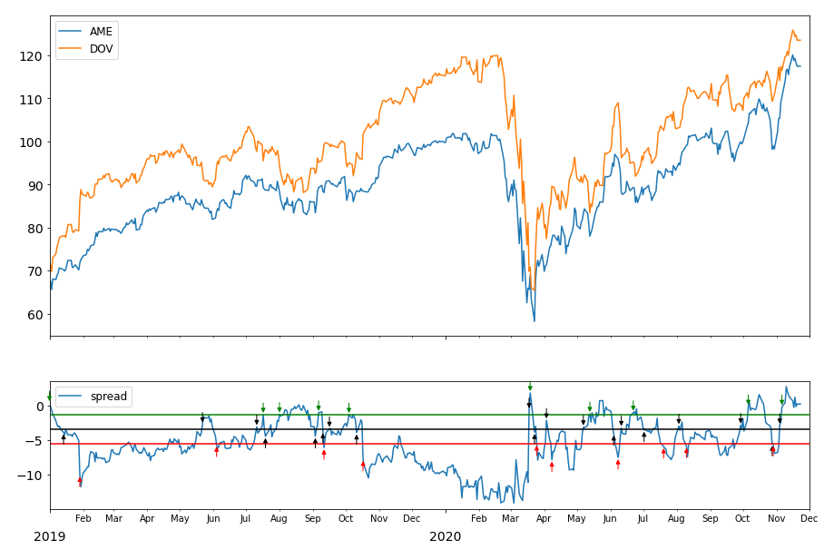
An example of pair trading Ametek Inc. (AME) and Dover Corp. (DOV) from January 2nd, 2019 to date. The green line defines the boundary for U-trades and the red line defines the boundary for L-trades. They equally deviate from the cointegration error mean (the black line).
Mean First-passage Time of an AR(1) Process
Consider a stationary AR(1) process:
where \(-1 < \phi < 1\), and \(\xi_t \sim N(0, \sigma_{\xi}^2) \quad \mathrm{i.i.d}\). The mean first-passage time over interval \(\lbrack a, b \rbrack\) of \(Y_t\), starting at initial state \(y_0 \in \lbrack a, b \rbrack\), which is denoted by \(E(\mathcal{T}_{a,b}(y_0))\), is given by
This integral equation can be solved numerically using the Nyström method, i.e. by solving the following linear equations:
where \(E_n(\mathcal{T}_{a,b}(u_0))\) is a discretized estimate of the integral, and the Gaussian kernel function \(K(u_i, u_j)\) is defined as:
and the weight \(w_j\) is defined by the trapezoid integration rule:
The time complexity for solving the above linear equation system is \(O(n^3)\) (see here
for an introduction of the time complexity of numpy.linalg.solve), which is the most time-consuming part of this
procedure.
Minimum Total Profit (MTP)
The MTP of U-trades within a specific trading horizon \(\lbrack 0, T \rbrack\) is defined by:
where \(TD_U\) is the trade duration and \(I_U\) is the inter-trade interval.
From the definition, the MTP is simultaneously determined by \(TD_U\) and \(I_U\), both of which can be derived from the mean first-passage time. Also, it is already known that \(U\) is the minimum profit per U-trade, so \(\frac{T}{TD_U + I_U} - 1\) can be used to estimate the number of U-trades. Following the assumption that the de-meaned cointegration error follows an AR(1) process:
Since the core idea of the approach is to “fade the spread” at \(U\), the trade duration can be defined as the average time of the cointegration error to pass 0 for the first time given that its initial value is \(U\). Thus using the definition of the mean first-passage time of the cointegration error process:
The inter-trade interval is defined as the average time of the de-meaned cointegration error to pass \(U\) the first time given its initial value is 0.
Under the assumption that the cointegration error follows a stationary AR(1) process, the standard deviation of the fitted residual \(\sigma_a\) and the standard deviation of the cointegration error \(\sigma_{\varepsilon}\) has the following relationship:
The following stylized fact helped approximate the infinity limit for both integrals: for a stationary AR(1) process \(\{ \varepsilon_t \}\), the probability that the absolute value of the process \(\vert \varepsilon_t \vert\) is greater than 5 times the standard deviation of the process \(5 \sigma_{\varepsilon}\) is close to 0. Therefore, \(5 \sigma_{\varepsilon}\) will be used as an approximation of the infinity limit in the integrals.
Optimize the Pre-Set Boundaries that Maximizes MTP
Based on the above definitions, the numerical algorithm to optimize the pre-set boundaries that maximize MTP could be given as follows.
Perform Engle-Granger or Johansen test (see here) to derive the cointegration coefficient \(\beta\).
Fit the cointegration error \(\varepsilon_t\) to an AR(1) process and retrieve the AR(1) coefficient and the fitted residual.
Calculate the standard deviation of cointegration error (\(\sigma_{\varepsilon}\)) and the fitted residual (\(\sigma_a\)).
Generate a sequence of pre-set upper bounds \(U_i\), where \(U_i = i \times 0.01, \> i = 0, \ldots, b/0.01\), and \(b = 5 \sigma_{\varepsilon}\).
For each \(U_i\),
Calculate \({TD}_{U_i}\).
Calculate \(I_{U_i}\). Note: this is the main bottleneck of the optimization speed.
Calculate \(MTP(U_i)\).
Find \(U^{*}\) such that \(MTP(U^{*})\) is the maximum.
Set a desired minimum profit \(K \geq U^{*}\) and calculate the number of assets to trade according to the following equations:
Trading the Strategy
After applying the above-described optimization rules, the output is optimal levels to enter and exit trades as well as number of shares to trade per leg of the cointegration pair. These outputs can be used in the Minimum Profit Trading Rule described in the Spread Trading section of the documentation.
Implementation
Example
# Importing packages
import pandas as pd
from arbitragelab.cointegration_approach.minimum_profit import MinimumProfit

# Read price series data, set date as index
data = pd.read_csv('X_FILE_PATH.csv', parse_dates=['Date'])
data.set_index('Date', inplace=True)

# Initialize the optimizer
optimizer = MinimumProfit()

# Set the training dataset
optimizer = optimizer.set_train_dataset(data)

# Run an Engle-Granger test to retrieve cointegration coefficient
beta_eg, epsilon_t_eg, ar_coeff_eg, ar_resid_eg = optimizer.fit(use_johansen=False)

# Optimize the pre-set boundaries, retrieve optimal upper bound, optimal minimum total profit,
# and number of trades.
optimal_ub, _, _, optimal_mtp, optimal_num_of_trades = optimizer.optimize(ar_coeff_eg,
                                                                          epsilon_t_eg,
                                                                          ar_resid_eg,
                                                                          len(train_df))

# Generate optimal trading levels and number of shares to trade
num_of_shares, optimal_levels = optimizer.get_optimal_levels(optimal_ub,
                                                             minimum_profit,
                                                             beta_eg,
                                                             epsilon_t_eg)
Research Notebooks
Research Article
Presentation Slides