Note
The following documentation closely follows a book by Simão Moraes Sarmento and Nuno Horta: A Machine Learning based Pairs Trading Investment Strategy.
Warning
In order to use this module, you should additionally install TensorFlow v2.8.0. and Keras v2.3.1. For more details, please visit our ArbitrageLab installation guide.
ML Based Pairs Selection
The success of a Pairs Trading strategy highly depends on finding the right pairs. But with the increasing availability of data, more traders manage to spot interesting pairs and quickly profit from the correction of price discrepancies, leaving no margin for the latecomers. On the one hand, if the investor limits its search to securities within the same sector, as commonly executed, he is less likely to find pairs not yet being traded in large volumes. If on the other hand, the investor does not impose any limitation on the search space, he might have to explore an excessive number of combinations and is more likely to find spurious relations.
To solve this issue, this work proposes the application of Unsupervised Learning to define the search space. It intends to group relevant securities (not necessarily from the same sector) in clusters, and detect rewarding pairs within them, that would otherwise be harder to identify, even for the experienced investor.
Proposed Pairs Selection Framework
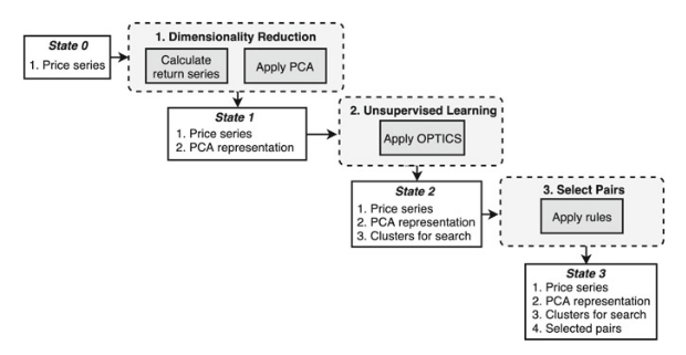
Framework diagram from A Machine Learning based Pairs Trading Investment Strategy. by Simão Moraes Sarmento and Nuno Horta.
Dimensionality Reduction
The main objectives in this step are:
Extracting common underlying risk factors from securities returns
Producing a compact representation for each security (stored in the variable ‘feature_vector’)
In this step the number of features, k, needs to be defined. A usual procedure consists of analyzing the proportion of the total variance explained by each principal component, and then using the number of components that explain a fixed percentage, as in Avellaneda M, Lee JH (2010). However, given that in this framework an Unsupervised Learning Algorithm is applied, the approach adopted took the data dimensionality problem as a major consideration. High data dimensionality presents a dual problem.
The first being that in the presence of more attributes, the likelihood of finding irrelevant features increases.
The second is the problem of the curse of dimensionality.
This term is introduced by Bellman (1966) to describe the problem caused by the exponential increase in volume associated with adding extra dimensions to Euclidean space. This has a tremendous impact when measuring the distance between apparently similar data points that suddenly become all very distant from each other. Consequently, the clustering procedure becomes very ineffective.
According to Berkhin (2006), the effect starts to be severe for dimensions greater than 15. Taking this into consideration, the number of PCA dimensions is upper bounded at this value and is chosen empirically.
Warning
Usually the number of components for dimensionality reduction is chosen purely to maximize the amount of variance in the final lower dimensional representation. In this module’s case, there is a need to balance the amount of variance represented and at the same time have the final representation remain dense enough (in a euclidean geometrical sense) for the clustering algorithm to detect any groupings. Thus as mentioned above the initial number of components is suggested to be 15 and slowly moved lower.
Implementation
Unsupervised Learning
The main objective in this step is to identify the optimal cluster structure from the compact representation previously generated, prioritizing the following constraints;
No need to specify the number of clusters in advance
No need to group all securities
No assumptions regarding the clusters’ shape.
The first method is to use the OPTICS clustering algorithm and letting the built-in automatic procedure to select the most suitable \(\epsilon\) for each cluster.
The second method is to use the DBSCAN clustering algorithm. This is to be used when the user has domain specific knowledge that can enhance the results given the algorithm’s parameter sensitivity. A possible approach to finding \(\epsilon\) described in Rahmah N, Sitanggang S (2016) is to inspect the knee plot and fix a suitable \(\epsilon\) by observing the global curve turning point.
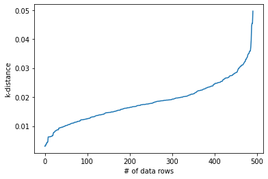
An example plot of the k-distance ‘knee’ graph
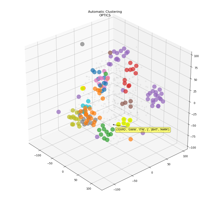
3D plot of the clustering result using the OPTICS method.
Implementation
Select Spreads
Note
In the original paper Pairs Selection module was a part of ML Pairs Trading approach. However, the user may want to use pairs selection rules without applying DBSCAN/OPTICS clustering. That is why, we decided to split pairs/spreads selection and clustering into different objects which can be used separately or together if the user wants to repeat results from the original paper.
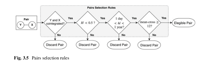
The rules selection flow diagram from A Machine Learning based Pairs Trading Investment Strategy. by Simão Moraes Sarmento and Nuno Horta.
The rules that each pair needs to pass are:
The pair’s constituents are cointegrated. Literature suggests cointegration performs better than minimum distance and correlation approaches
The pair’s spread Hurst exponent reveals a mean-reverting character. Extra layer of validation.
The pair’s spread diverges and converges within convenient periods.
The pair’s spread reverts to the mean with enough frequency.
To test for cointegration, the framework proposes the application of the Engle-Granger test, due to its simplicity. One critic Armstrong (2001) points at the Engle-Granger test sensitivity to the ordering of variables. It is a possibility that one of the relationships will be cointegrated, while the other will not. This is troublesome because we would expect that if the variables are truly cointegrated the two equations will yield the same conclusion.
To mitigate this issue, the original paper proposes that the Engle-Granger test is run for the two possible selections of the dependent variable and that the combination that generated the lowest t-statistic is selected. Further work in Hoel (2013) adds on, “the unsymmetrical coefficients imply that a hedge of long / short is not the opposite of long / short , i.e. the hedge ratios are inconsistent”.
A better solution is proposed and implemented, based on Gregory et al. (2011) to use orthogonal regression – also referred to as Total Least Squares (TLS) – in which the residuals of both dependent and independent variables are taken into account. That way, we incorporate the volatility of both legs of the spread when estimating the relationship so that hedge ratios are consistent, and thus the cointegration estimates will be unaffected by the ordering of variables.
Hudson & Thames research team has also found out that optimal (in terms of cointegration tests statistics) hedge ratios are obtained by minimizng spread’s half-life of mean-reversion. Alongside this hedge ration calculation method, there is a wide variety of algorithms to choose from: TLS, OLS, Johansen Test Eigenvector, Box-Tiao Canonical Decomposition, Minimum Half-Life, Minimum ADF Test T-statistic Value.
Note
More information about the hedge ratio methods and their use can be found in the Hedge Ratio Calculations section of the documentation.
Secondly, an additional validation step is also implemented to provide more confidence in the mean-reversion character of the pairs’ spread. The condition imposed is that the Hurst exponent associated with the spread of a given pair is enforced to be smaller than 0.5, assuring the process leans towards mean-reversion.
In third place, the pair’s spread movement is constrained using the half-life of the mean-reverting process. In the framework paper the strategy built on top of the selection framework is based on the medium term price movements, so for this reason the spreads that either have very short (< 1 day) or very long mean-reversion (> 365 days) periods were not suitable.
Lastly, we enforce that every spread crosses its mean at least once per month, to provide enough liquidity and thus providing enough opportunities to exit a position.
Note
A more detailed explanation of the CointegrationSpreadSelector class and examples of use can be found in the Cointegration Rules Spread Selection section of the documentation.
Examples
# Importing packages
import pandas as pd
import numpy as np
from arbitragelab.ml_approach import OPTICSDBSCANPairsClustering
from arbitragelab.spread_selection import CointegrationSpreadSelector

# Getting the dataframe with time series of asset returns
data = pd.read_csv('X_FILE_PATH.csv', index_col=0, parse_dates = [0])

pairs_clusterer = OPTICSDBSCANPairsClustering(data)

# Price data is reduced to its component features using PCA
pairs_clusterer.dimensionality_reduction_by_components(5)

# Clustering is performed over feature vector
clustered_pairs = pairs_clusterer.cluster_using_optics(min_samples=3)

# Removing duplicates
clustered_pairs = list(set(clustered_pairs))

# Generated Pairs are processed through the rules mentioned above
spreads_selector = CointegrationSpreadSelector(prices_df=data,
                                               baskets_to_filter=clustered_pairs)
filtered_spreads = spreads_selector.select_spreads()

# Checking the resulting spreads
print(filtered_spreads)

# Generate a plot of the selected spread
spreads_selector.spreads_dict['AAL_FTI'].plot(figsize=(12,6))

# Generate detailed spread statistics
spreads_selector.selection_logs.loc[['AAL_FTI']].T
Research Notebooks
The following research notebook can be used to better understand the Pairs Selection framework described above.