Note
The following documentation closely follows a paper by Chen et al. (2012): Empirical investigation of an equity pairs trading strategy.
As well as a paper by Perlin, M. S. (2009): Evaluation of pairs-trading strategy at the Brazilian financial market.
And also a paper by Christopher Krauss (2015): Statistical arbitrage pairs trading strategies: Review and outlook.
Pearson Approach
After the distance approach was introduced in the paper by Gatev et al. (2006), a lot of research has been conducted to further develop the original distance approach. One of the adjustments is the Pearson correlation approach proposed by Chen et al.(2012). In this paper, the authors use the same data set and time frame as in the work by Gatev et al.(2006), but they used Pearson correlation on return level for forming pairs. In the formation period(5 years in the paper), pairwise return correlations for all pairs in the universe are calculated based on monthly return data. Then the authors construct a new variable, Return Divergence (\(D_{i j t}\)), to capture the return divergence between a single stock’s return and its pairs-portfolio returns:
where \(\beta\) denotes the regression coefficient of stock’s monthly return \(R_{i t}\) on its pairs-portfolio return \(R_{j t}\), and \(R_{f}\) is the risk-free rate.
The hypothesis in this approach is that if a stock’s return deviates from its pairs portfolio returns more than usual, this divergence is expected to be reversed in the next month. And the returns of this stock are expected to be abnormally high/low in comparison to other stocks.
Therefore, after calculating the return divergence of all the stocks, a long-short portfolio is constructed based on the long and short ratio given by the user.
Pairs Portfolio Formation
This stage of PearsonStrategy consists of the following steps:
Data preprocessing
As the method has to compute all of the pairs’ correlation values in the following steps, for \(m\) stocks, there are \(\frac{m*(m-1)}{2}\) correlations to be computed in the formation period. As the number of observations for the correlations grows exponentially with the number of stocks, this estimation is computationally intensive.
Therefore, to reduce the computation burden, this method uses monthly stock returns data in the formation period (ex. 60 monthly stock returns if the formation period is 5 years). If the daily price data is given, the method calculates the monthly returns before moving into the next steps.
Finding pairs
For each stock, the method finds \(n\) stocks with the highest correlations to the stock as its pairs using monthly stock returns. After pairs are formed, returns of pairs, which refer to as pairs portfolios in the paper, are needed to create \(beta\) in the following step. Therefore, this method uses two different weighting metrics in calculating the returns.
The first is an equal-weighted portfolio. The method by default computes the pairs portfolio returns as the equal-weighted average returns of the top n pairs of stocks. The second is a correlation-weighted portfolio. If this metric is chosen, the method uses the stock’s correlation values to each of the pairs and forms a portfolio weighted by these values and the weights are calculated by the formula:
where \(w_{k}\) is the weight of stock k in the portfolio and \(\rho_{i}\) is a correlation of the stock and one of its pairs.
Calculating beta
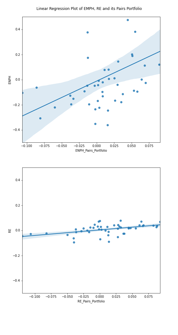
After pairs portfolio returns are calculated, the method derives beta from the monthly return of the stock and its pairs portfolio. By using linear regression, setting stock return as independent variable and pairs portfolio return as the dependent variable, the methods set beta as a regression coefficient. Then the beta is stored in a dictionary for future uses in trading. Below is a figure showing two stocks with high beta (ENPH) and low beta (RE).
Implementation
Trading Signal Generation
After calculating the betas for all of the stocks in the formation period, the next step is to generate trading signals by calculating the return divergence for each of the stocks. In this method, test data is not necessarily required if only a trading signal for the last month of the formation period is needed. However, if one wants to see the backtesting results of the method and test with test data, a successive dataset after the formation period is required to generate the proper trading signals. The steps are as follows:
Data Preprocessing
The same data preprocessing is done with the formation period as the data needs to be in the same format. As in the formation period, the risk-free rate can be given in the form of either a float number or a series of data.
Calculating the Return Divergence
For every month of test data, starting from the very last month of the train data, return divergences are calculated with the beta created in the formation period. The equation for calculating the return divergence is in the first section of this documentation. Note that while the return divergence between a portfolio of \(n\) most-highly correlated stocks with stock i and stock \(i\) is used as a sorting variable, only individual stock \(i\) enters the portfolio construction, not those \(n\) stocks. The portfolio of those \(n\) stocks only serves as a benchmark for portfolio sorting.
Finding Trading Signals
Then, all stocks are sorted in descending order based on their previous month’s return divergence. If the percentages of long and short stocks are given, say \(p\%\) and \(q\%\), the top \(p\%\) of the sorted stocks are chosen for the long stocks and the bottom \(q\%\) of the sorted stocks are chosen for the short stocks. If a user wants to construct a dollar-neutral portfolio, one should choose the same percentage for \(p\) and \(q\). Finally, a new dataframe is created with all of the trading signals: 1 if a stock is in a long position, -1 if it is in a short position and 0 if it does not have any position.
Implementation
Results output
The PearsonStrategy class contains multiple methods to get results in the desired form.
Functions that can be used to get data:
get_trading_signal() outputs trading signal in monthly basis. 1 for a long position, -1 for a short position and 0 for closed position.
get_beta_dict() outputs beta, a regression coefficients for each stock, in the formation period.
get_pairs_dict() outputs top n pairs selected during the formation period for each of the stock.
Implementation
Examples
Code Example
# Importing packages
import pandas as pd
from arbitragelab.distance_approach.pearson_distance_approach import PearsonStrategy

# Getting the dataframe with price time series for a set of assets
data = pd.read_csv('X_FILE_PATH.csv', index_col=0, parse_dates = [0])
risk_free = pd.read_csv('Y_FILE_PATH.csv', index_col=0, parse_dates = [0])

# Dividing the dataset into two parts - the first one for pairs formation
train_data = data.loc[:'2019-01-01']
risk_free_train = risk_free.loc[:'2019-01-01']

# And the second one for signals generation
test_data = data.loc['2019-01-01':]
risk_free_test = risk_free.loc['2019-01-01':]

# Performing the portfolio formation stage of the PearsonStrategy
# Choosing top 50 pairs to calculate beta and set other parameters as default
strategy = PearsonStrategy()
strategy.form_portfolio(train_data, risk_free_train, num_pairs=50)

# Checking a list of beta that were calculated
beta_dict = strategy.get_beta_dict()

# Checking a list of pairs in the formation period
pairs = strategy.get_pairs_dict()

# Now generating signals for formed pairs and beta
strategy.trade_portfolio(test_data, risk_free_test)

# Checking generated trading signals in the test period
signals = strategy.get_trading_signal()
Research Notebooks
The following research notebook can be used to better understand the Pearson approach described above.