Mispricing Index Copula Trading Strategy
Note
The following strategy closely follows the implementations:
Pairs trading with copulas. (2014) by Xie, W., Liew, R.Q., Wu, Y. and Zou, X.
The profitability of pairs trading strategies: distance, cointegration and copula methods. (2016) by Rad, H., Low, R.K.Y. and Faff, R.
Note
The authors claimed a relatively robust 8-10% returns from this strategy in the formation period (6 mo).
We are pretty positive that the rules proposed in the paper were implemented correctly in the MPICopulaTradingRule
module with thorough unit testing on every possible case, and thus it is very unlikely that we made logical mistakes.
However the P&L is very sensitive to the opening and exiting logic and parameter values, input data and copula choice,
and it cannot lead to the claimed returns, after trying all the possible interpretations of ambiguities.
We found out that using an AND for opening and OR for exiting lead to a much less sensitive strategy and generally leads to a much better performance, and we provide such an option in the module.
We still implement this module for people who intend to explore possibilities with copula, however the user should be aware of the nature of the proposed framework. Interested reader may read through the Possible Issues part and see where this strategy can be improved, and is encouraged to make changes in the source code, where we grouped the exit and open logic in one function for ease of alteration.
Introduction to the Strategy Concepts
For convenience, the mispricing index implemented in the strategy will be referred to MPI when no ambiguity arises.
A Quick Review of the Basic Copula Strategy
Before we introduce the MPI strategy, let’s recall the basic copula strategy and understand its pros and cons.
The basic copula strategy proposed by [Liew et al. 2013] works with price series (or log-price series, which has identical suggested trading signals under the copula framework) and looks at conditional probabilities. For example, if \(P(X \le x_t | Y = y_t)\) is small for stock pair \((X, Y)\) with prices \((x_t, y_t)\), then stock \(X\) is considered undervalued given the current price of \(Y\). Then we derive long/short positions regarding the spread based on this conditional probability. This conditional probability is calculated from some copula fitted to the training data, and generally other models cannot produce this value.
Although this approach is in general reasonably sound, it has one critical drawback, that the price series is not in general stationary. For example, if one adopt the assumption that stocks move in a lognormal (One may also argue that such assumption can be quite situational. We won’t get into the details here.) fashion, then almost surely the price will reach any given level with enough time.
This implies that, if the basic copula framework was working on two stocks that have an upward(or downward) drift in the trading period, it may go out of range of the training period, and the conditional probabilities calculated from which will always be extreme values as \(0\) and \(1\), bringing in nonsense trading signals. One possible way to overcome this inconvenience is to keep the training set up to date so it is less likely to have new prices out of range. Another way is to work with a more likely stationary time series, for example, returns.
How is the MPI Strategy Constructed?
At first glance, the MPI strategy documented in [Xie et al. 2016] looks quite bizarre. However, it is reasonably consistent when one goes through the logic of its construction: In order to use returns to generate trading signals, one needs to be creative about utilizing the information. It is one thing to know the dependence structure of a pair of stocks, it is another thing to trade based on it because intrinsically stocks are traded on prices, not returns.
If one regards using conditional probabilities as a distance measure, then it is natural to think about how far the returns have cumulatively driven the prices apart (or together), thereby introducing trading opportunities.
Hence we introduce the following concepts for the strategy framework:
Mispricing Index
MPI is defined as the conditional probability of returns, i.e.,
for stocks \((X, Y)\) with returns random variable at day \(t\): \((R_t^X, R_t^Y)\) and returns value at day \(t\): \((r_t^X, r_t^Y)\). Those two values determine how mispriced each stock is, based on that day’s return. Note that so far only one day’s return information contributes, and we want to add it up to cumulatively use returns to gauge how mispriced the stocks are. Therefore we introduce the flag series:
Flag and Raw Flag
A more descriptive name than flag, in my opinion, would be cumulative mispricing index. The raw flag series (with a star) is the cumulative sum of daily MPIs minus 0.5, i.e.,
Or equivalently
If one plots the raw flags series, they look quite similar to cumulative returns from their price series, which is what they were designed to do: Accumulate information from daily returns to reflect information on prices. Therefore, you may consider it as a fancy way to represent the returns series.
However, the real flag series (without a star, \(FlagX(t)\), \(FlagY(t)\)) will be reset to 0 whenever there is an exiting signal, which brings us to the trading logic.
Trading Logic
Default Opening and Exiting Rules
The authors propose a dollar-neutral trade scheme worded as follows:
Suppose stock \(X\), \(Y\) are associated with \(FlagX\), \(FlagY\) respectively.
Opening rules: (\(D = 0.6\) in the paper)
When \(FlagX\) reaches \(D\), short \(X\) and buy \(Y\) in equal amounts. (\(-1\) Position)
When \(FlagX\) reaches \(-D\), short \(Y\) and buy \(X\) in equal amounts. (\(1\) Position)
When \(FlagY\) reaches \(D\), short \(Y\) and buy \(X\) in equal amounts. (\(1\) Position)
When \(FlagY\) reaches \(-D\), short \(X\) and buy \(Y\) in equal amounts. (\(-1\) Position)
Exiting rules: (\(S = 2\) in the paper)
If trades are opened based on \(FlagX\), then they are closed if \(FlagX\) returns to zero or reaches stop-loss position \(S\) or \(-S\).
If trades are opened based on \(FlagY\), then they are closed if \(FlagY\) returns to zero or reaches stop-loss position \(S\) or \(-S\).
After trades are closed, both \(FlagX\) and \(FlagY\) are reset to \(0\).
The rationale behind the dollar-neutral choice might be that (the authors did not mention this), because the signals are generated by returns, it makes sense to “reset” returns when entering into a long/short position.
Ambiguities
The authors did not specify what will happen if the following occurs:
When \(FlagX`reaches :math:`D\) (or \(-D\)) and \(FlagY\) reaches \(D\) (or \(-D\)) together.
When in a long(or short) position, receives a short(or long) trigger.
When receiving an opening and exiting signal together.
When the position was open based on \(FlagX\) (or \(FlagY\)), \(FlagY\) (or \(FlagX\)) reaches \(S\) or \(-S\).
Here is our take on the above issues:
Do nothing.
Change to the trigger position. For example, a long position with a short trigger will go short.
Go for the exiting signal.
Do nothing.
Choices for Open and Exit Logic
The above default logic is essentially an OR-OR logic for open and exit: When at least one of the 4 open conditions is satisfied, an open signal (long or short) is triggered; Similarly for the exit logic, to exit only one of them needs to be satisfied. The opening trigger is in general too sensitive and leads to too many trades, and [Rad et al. 2016] suggested using AND-OR logic instead. Thus, to achieve more flexibility, we allow the user to choose AND, OR for both open and exit logic and hence there are 4 possible combinations. Based on our tests we found AND-OR to be the most reasonable choice in general, but in certain situations other choices may have an edge.
The default is OR-OR, as suggested in [Xie et al. 2014], and you can switch to other logic in the get_positions_and_flags method
by setting open_rule and exit_rule to your own liking.
For instance open_rule='and', exit_rule='or'.
Note
There are some nuiances on how the logic is carried.
In the paper [Xie et al. 2014], they tracked which stock led to opening of a position, and it influences the exit.
This tracking procedure makes no sense for other 3 trading logics.
The variable open_based_on is present in lower level functions that are (python) private, and they track which stock triggered the last
opening.
Thus this variable is not used (although still calculated, but it is likely incorrect) when using other logic.
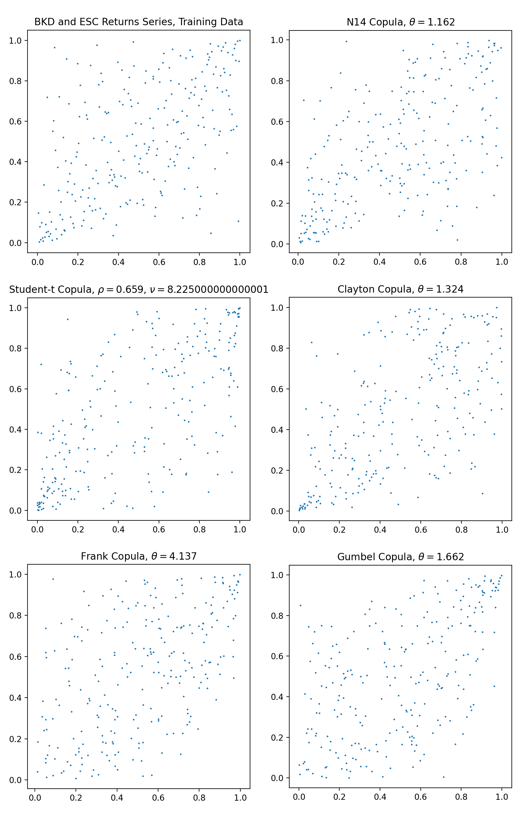
Sampling from the various fitted copulas, and plot the empirical density from training data from BKD and ESC.
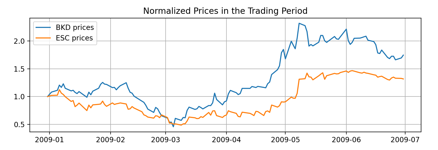
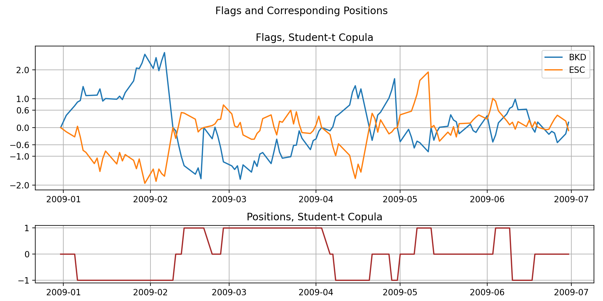

A visualised output of flags, positions and units to hold using a Student-t copula. The stock pair considered is BKD and ESC.
Implementation
Example
# Importing the module and other libraries
from arbitragelab.trading.copula_strategy_mpi import MPICopulaTradingRule
from arbitragelab.copula_approach import construct_ecdf_lin
from arbitragelab.copula_approach.archimedean import N14
import matplotlib.pyplot as plt
import pandas as pd

# Instantiating the module
CSMPI = MPICopulaTradingRule(opening_triggers=(-0.6, 0.6), stop_loss_positions=(-2, 2))

# Loading the data in prices of stock X and stock Y
prices = pd.read_csv('FILE_PATH' + 'stock_X_Y_prices.csv').set_index('Date').dropna()

# Convert prices to returns
returns = CSMPI.to_returns(prices)

# Split data into train and test sets
training_len = int(len(prices) * 0.7)
returns_train = returns.iloc[:training_len, :]
returns_test = returns.iloc[training_len:, :]
prices_train = prices.iloc[:training_len, :]
prices_test = prices.iloc[training_len:, :]

# Adding the N14 copula (it can be fitted with tools from the Copula Approach)
cop = N14(theta=2)
CSMPI.set_copula(cop)

# Constructing cdf for x and y
cdf_x = construct_ecdf_lin(returns['BKD'])
cdf_y = construct_ecdf_lin(returns['ESC'])
CSMPI.set_cdf(cdf_x, cdf_y)

# Forming positions and flags using trading data, assuming holding no position initially.
# Default uses OR-OR logic for open-exit.
positions, flags = CSMPI.get_positions_and_flags(returns=returns_test)

# Use AND-OR logic.
positions_and_or, flags_and_or = CSMPI.get_positions_and_flags(returns=returns_test,
                                                               open_rule='and',
                                                               exit_rule='or')

# Changing the positions series to units to hold for
# a dollar-neutral strategy for $10000 investment
units = CSMPI.positions_to_units_dollar_neutral(prices_df=prices_test,
                                                positions=positions,
                                                multiplier=10000)
Possible Issues
The following are critiques for the default strategy. For a thorough comparison in large amounts of stocks across several decades, read For the AND-OR strategy, read more in [Rad et al. 2016] on comparisons with other common strategies, using the AND-OR logic.
The default strategy’s outcome is quite sensitive to the values of opening and exiting triggers to the point that a well-fitted copula with a not-so-good set of parameters can actually lose money.
The trading signal is generated from the flags series, and the flags series will be calculated from the copula that we use to model. Therefore the explainability suffers. Also, it is based on the model in second order, and therefore the flag series and the suggested positions will be quite different across different copulas, making it not stable and not directly comparable mutually.
The way the flags series are defined does not handle well when both stocks are underpriced/overpriced concurrently.
Because flags will be reset to 0 once there is an exiting signal, it implicitly models the returns as martingales that do not depend on the current price level of the stock itself and the other stock. Such an assumption may be situational, and the user should be aware. (White noise returns do not imply that the prices are well cointegrated.)
The strategy is betting the flags series having dominating mean-reversion behaviors, for a pair of cointegrated stocks. It is not mathematically clear what justifies the rationale.
If accumulating mispricing index is basically using returns to reflect prices, and the raw flags look basically the same as normalized prices, why not just directly use normalized prices instead?
Research Notebooks
The following research notebook can be used to better understand the copula strategy described above.