Note

The following implementations and documentation closely follow the below work:

Liu, J. and Timmermann, A., 2013. Optimal convergence trade strategies.

Optimal Convergence

Introduction

Convergence trades resemble the standard long-short arbitrage strategy popular in industry and covered in academic studies. Conventionally, such strategies take positions of equal size but opposite signs either in portfolio weight or in number of shares. This seems intuitively reasonable and ensures that future liabilities offset. However, as shown in the paper, such delta neutral strategies will typically not be optimal.

The objective of optimally trading off risk and returns can lead to quite different solutions compared with the standard arbitrage objective assumed in convergence trades. Traditional arbitrage strategies and/or delta neutral convergence trades are designed to explore long-term arbitrage opportunities but usually do not exploit the short-run risk-return trade-off optimally. By placing arbitrage opportunities in the context of a portfolio maximization problem, the optimal convergence strategy accounts for both arbitrage opportunities and diversification benefits.

Modelling

In the paper, the authors assume that there is a riskless asset that pays a constant rate of return, \(r\). A risky asset trading at the price \(P_{mt}\) represents the market index. This follows a geometric random walk process,

\[\frac{d P_{m t}}{P_{m l}}=\left(r+\mu_{m}\right) d t+\sigma_{m} d B_{t}\]

where the market risk premium, \(\mu_{m}\), and market volatility, sigma_{m}`, are both constant, and \(B_t\) is a standard Brownian motion.

In addition to the risk-free asset and the market index, the authors assume the presence of two risky assets whose prices \(P_{it}, i = 1,2\), evolve according to the equations

\[\begin{split}\begin{array}{l} \frac{d P_{1 t}}{P_{1 t}}=\left(r+\beta \mu_{m}\right) d t+\beta \sigma_{m} d B_{t}+\sigma d Z_{t}+b d Z_{1 t} -\lambda_{1} x_{t} d t \\ \frac{d P_{2 t}}{P_{2 t}}=\left(r+\beta \mu_{m}\right) d t+\beta \sigma_{m} d B_{t}+\sigma d Z_{t}+b d Z_{2 t} +\lambda_{2} x_{t} d t \end{array}\end{split}\]

where \(\lambda_1\), \(\lambda_2\), \(\beta\), \(b\), and \(\sigma\) are constant parameters. \(Z_t\) and \(Z_{it}\) are standard Brownian motions, and \(B_t\) , \(Z_t\) , and \(Z_{it}\) are all mutually independent for \(i = 1,2\).

In the above equations, \(\beta \sigma_m d B_t\) represents exposure to the market risk, whereas \(\sigma d Z_{t}+b d Z_{t}\) represents idiosyncratic risks. It is standard to assume that idiosyncratic risks are independent across different stocks with the market risk representing the only source of correlation among different assets.

\(x_t\) represents pricing errors in our model and is the difference between the logarithms of the two asset prices, \(p_{it} = \ln P_{it}\) ,

\[x_t = p_{1t} − p_{2t} =\ln\bigg(\frac{P_{1t}}{P_{2t}}\bigg)\]

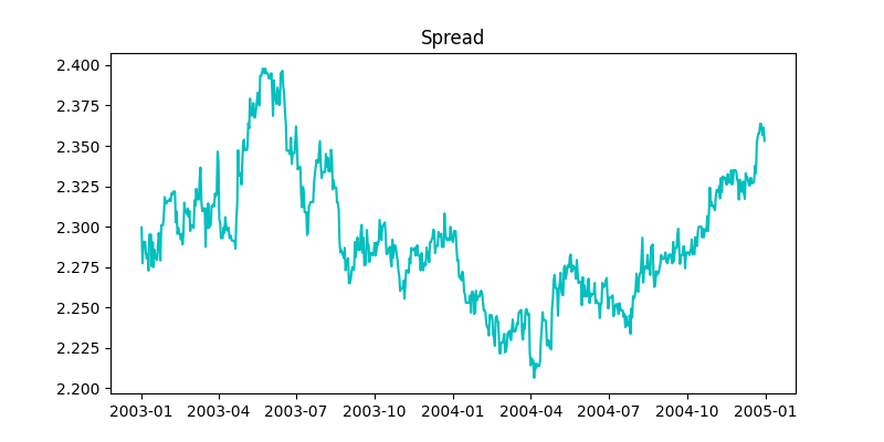
Constructed spread for the Royal Dutch - Shell pair.

The authors make a key assumption here, that \(\lambda_1 + \lambda_2 > 0\). This implies that \(x_t\) is stationary and the logarithms of the prices are cointegrated with cointegrating vector \((1,−1)\).

The cointegration setup captures the feature that two assets with identical payoffs can trade at different prices. Examples include pairs of stocks that have the same claim to dividends and identical voting rights but are traded in different markets and two stocks with the same payoffs, such as the target and acquirer stocks in a merger.

\(−\lambda_1 x_t\) and \(\lambda_2 x_t\) capture the absolute mispricing of each asset relative to CAPM. For further information regarding the utility of \(\lambda\)’s, interested readers can refer to Section 1.1 in the paper.

Cointegration and relative mispricing

\(x_t\) represents the relative mispricing between both assets. This is considered stationary and the dynamics of this term is given by,

\[d x_{t}=-\lambda_{x} x_{t} d t+b_{x} d Z_{x t}\]

where,

\[\begin{split}\begin{array}{c} \lambda_{x}=\lambda_{1}+\lambda_{2}, \\ b_{x} d Z_{x t}=b d Z_{1 t}-b d Z_{2 t}, \\ b_x = \sqrt 2 b \end{array}\end{split}\]

In this paper, the authors considered two cases for both the unconstrained and constrained(delta neutral) portfolios. The first case deals with recurring arbitrage opportunities, the price differential, \(x_t\) , only spends an infinitesimally short time at zero, is characterized at all times by the dynamics in the above equation, and so follows a stationary process. In the second case (“nonrecurring arbitrage opportunities”), any price difference is temporary and gets permanently eliminated the first time the two prices converge and \(x_t = 0\). In this case, the price dynamics is subject to the additional restriction that \(x_{\tau + \delta} = 0\) for all \(\delta ≥ 0\), where \(\tau = min(t : x_t = 0)\) is a stopping time. In this case, prices remain identical after they converge. The optimal portfolio weights are different for these cases.

In the absence of intermediate consumption, the investor’s wealth, \(W_t\) , evolves according to the process,

\[\begin{split}\begin{aligned} d W_{t}=& W_{t}\left(r d t+\phi_{m t}\left(\frac{d P_{m t}}{P_{m t}}-r d t\right)+\phi_{1 t} \left(\frac{d P_{1 t}}{P_{1 t}}-r d t\right)+\phi_{2 t}\left(\frac{d P_{2 t}}{P_{2 t}}-r d t\right)\right) \\ =& W_{t}\left(r d t+\left(\phi_{m t}+\beta\left(\phi_{1 t}+\phi_{2 t}\right)\right)\left(\mu_{m} d t+\sigma_{m} d B_{t}\right)\right.\\ &+\phi_{1 t}\left(\sigma d Z_{t}+b d Z_{1 t}-\lambda_{1} x_{t} d t\right) \\ &\left.+\phi_{2 t}\left(\sigma d Z_{t}+b d Z_{2 t}+\lambda_{2} x_{t} d t\right)\right) . \end{aligned}\end{split}\]

We assume that the investor maximizes the expected value of a power utility function defined over terminal wealth, \(W_T\). The investor’s value function is given by

\[J(t, x, W)=\frac{1}{1-\gamma} \mathrm{E}_{t}\left[W_{T}^{*(1-\gamma)}\right]\]

where \(W^{*}_T\) is the wealth at time \(T\) obtained by the optimal trading strategy with \(W_t = W\) and \(x_t = x\) at time \(t\).

Unconstrained Optimal Investment Strategies

For the continuing cointegrated price process (recurring arbitrage opportunities), we get a closed-form solutions for the optimal portfolio weights.

The optimal weights on the market portfolio, \(\phi_{m t}^{*}\) , and the individual assets, \((\phi_{1 t}^{*}, \phi_{2 t}^{*})\), are given by

\[\begin{split}\begin{array}{c} \phi_{m t}^{*}=\frac{\mu_{m}}{\gamma \sigma_{m}^{2}}-\left(\phi_{1 t}^{*}+\phi_{2 t}^{*}\right) \beta \\ \left(\begin{array}{c} \phi_{1 t}^{*} \\ \phi_{2 t}^{*} \end{array}\right)=\frac{1}{\gamma\left(2 \sigma^{2}+b^{2}\right) b^{2}}\left(\begin{array}{cc} \sigma^{2}+b^{2} & -\sigma^{2} \\ -\sigma^{2} & \sigma^{2}+b^{2} \end{array}\right)\left(\begin{array}{c} -\lambda_{1}+b^{2} C(t) \\ \lambda_{2}-b^{2} C(t) \end{array}\right) \ln \left(\frac{P_{1 t}}{P_{2 t}}\right) \end{array}\end{split}\]

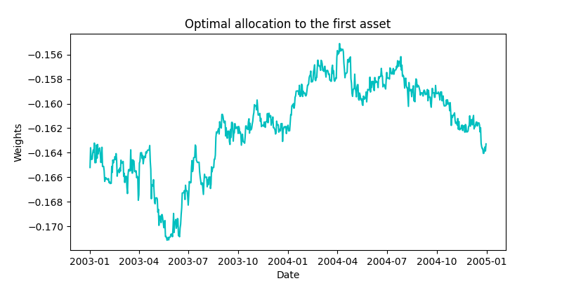
Optimal Portfolio Weights for the first asset in the Royal Dutch - Shell pair.

Optimal Portfolio Weights for the second asset in the Royal Dutch - Shell pair.

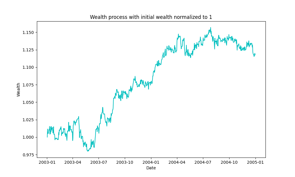
Total wealth of the portfolio with Optimal Portfolio Weights strategy.

Delta Neutral Strategy

In the model considered in the paper, where the two stocks are assumed to have identical market betas, delta neutrality directly translates into the constraint \(\phi_{1t} = −\phi_{2t}\). The authors suggest that the best way to achieve a delta neutral position is to use the market index to hedge away the market exposure in the mispriced assets. Using mispriced assets alone to achieve delta neutrality will necessarily underexploit opportunities offered by mispricing in the individual stocks.

For the continuing cointegrated price process (recurring arbitrage opportunities), we get closed-form solutions.

\[\begin{split}\begin{array}{l} \check{\phi}_{m t}^{*}=\frac{\mu_{m}}{\gamma \sigma_{m}^{2}}, \\ \check{\phi}_{1 t}^{*}=\frac{-\left(\lambda_{1}+\lambda_{2}\right) \ln \left(\frac{P_{1 t}}{P_{2 t}}\right)+2 b^{2} D(t) \ln \left(\frac{P_{1 t}}{P_{2 t}}\right)}{2 \gamma b^{2}} \end{array}\end{split}\]

Note

The optimal strategy is delta neutral if \(\lambda_1 = \lambda_2\).

Delta Neutral Portfolio Weights for the first asset in the Royal Dutch - Shell pair.

Delta Neutral Portfolio Weights for the second asset in the Royal Dutch - Shell pair.

Total wealth of the portfolio with Delta Neutral strategy.

How to use this submodule

This submodule contains six public methods, of which two methods are necessary to calculate the optimal weights. The first method fit is for estimating the parameters of the model using training data, and the second method is for calculating the final optimal portfolio weights using evaluation data.

Model fitting

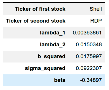
We input the training data to the fit method, which calculates the spread and the estimators of the parameters of the model.

Implementation

This module is a realization of the methodology in the following paper: Liu, J. and Timmermann, A., 2013. Optimal convergence trade strategies. The Review of Financial Studies, 26(4), pp.1048-1086.

class OptimalConvergence

This module models the optimal convergence trades under both recurring and nonrecurring arbitrage opportunities represented by continuing and “stopped” co-integrated price processes.

Along with delta neutral portfolios, this module also considers unconstrained optimal portfolios where the portfolio weights of both the stocks in the spread are calculated dynamically. Conventional long-short delta neutral strategies are generally suboptimal and it can be optimal to simultaneously go long (or short) in two mis-priced assets. Standard arbitrage strategies and/or delta neutral convergence trades are designed to explore long-term arbitrage opportunities but do typically not optimally exploit the short-run risk return trade-off. By placing arbitrage opportunities in the context of a portfolio maximization problem, this optimal convergence strategy accounts for both arbitrage opportunities and diversification benefits.

__init__()

Initializes the parameters of the module.

OptimalConvergence.fit(prices: DataFrame, mu_m: float, sigma_m: float, r: float, delta_t: float = 0.003968253968253968)

This method estimates the error-correction terms (lambda) using the inputted pricing data.

Parameters:

• prices – (pd.DataFrame) Contains price series of both stocks in spread.

• mu_m – (float) Market Risk Premium.

• sigma_m – (float) Market Volatility.

• r – (float) Interest Rate.

• delta_t – (float) Time difference between each index of data, calculated in years.

Tip

To view the estimated model parameters from training data, call the describe function.

OptimalConvergence.describe() → Series

Method returns values of instance attributes calculated from training data.

Returns:

(pd.Series) Series describing parameter values.

Optimal Unconstrained Portfolio Weights with recurring arbitrage opportunities

In this step we input the evaluation data and specify the utility function parameter \(\gamma\).

Warning

Please make sure the value of gamma is positive.

Implementation

OptimalConvergence.unconstrained_portfolio_weights_continuous(prices: DataFrame, gamma: float = 4) → tuple

Implementation of Proposition 1.

This method calculates the portfolio weights for the market asset and for both the stocks in the spread when there are no constraints put on values of lambda. We also assume a continuing cointegrated price process (recurring arbitrage opportunities), which gives closed-form solutions for the optimal portfolio weights.

If lambda_1 = lambda_2, from the portfolio weights outputted from this method phi_2 + phi_1 = 0, which implies delta neutrality. This follows Proposition 3 in the paper.

Parameters:

• prices – (pd.DataFrame) Contains price series of both stocks in spread.

• gamma – (float) Signifies investor’s attitude towards risk (positive float value).

Returns:

(tuple) Consists of three numpy arrays: weights for asset 1, asset 2, and market portfolio.

Delta Neutral Portfolio Weights with recurring arbitrage opportunities

In this step we input the evaluation data and specify the utility function parameter \(\gamma\).

Warning

Please make sure the value of gamma is positive.

Implementation

OptimalConvergence.delta_neutral_portfolio_weights_continuous(prices: DataFrame, gamma: float = 4) → tuple

Implementation of Proposition 2.

This method calculates the portfolio weights for the market asset and for both the stocks in the spread when the portfolio is constrained to be delta-neutral, where sum of portfolio weights of both the assets in the spread is zero. We also assume a continuing cointegrated price process (recurring arbitrage opportunities), which gives closed-form solutions for the optimal portfolio weights.

Parameters:

• prices – (pd.DataFrame) Contains price series of both stocks in spread.

• gamma – (float) Signifies investor’s attitude towards risk (positive float value).

Returns:

(tuple) Consists of three numpy arrays: weights for asset 1, asset 2, and market portfolio.

Wealth gain in continuous case

In this step we specify the utility function parameter \(\gamma\).

Warning

Please make sure the value of gamma is positive.

Implementation

OptimalConvergence.wealth_gain_continuous(gamma: float = 4, sigma: float = 0.15, b: float = 0.3, mu_m: float = 0.05, sigma_m: float = 0.35, r: float = 0.02, lambda_1: float = 0.52, lambda_2: float = -0.35) → array

Implementation of Proposition 4.

This method calculates the expected wealth gain of the unconstrained optimal strategy relative to the delta neutral strategy assuming a mis-pricing of the spread.

We take fixed values of spread between [0, 0.2]. The time to maturity is assumed to be 1 year for each value of spread.

The default values of the input parameters are taken according to the paper.

Parameters:

• gamma – (float) Signifies investor’s attitude towards risk (positive float value).

• b – (float) Model Parameter found in Equation (2-3) in the paper.

• mu_m – (float) Market Risk Premium.

• sigma_m – (float) Market Volatility.

• r – (float) Interest Rate.

• lambda_1 – (float) Parameter signifies relative liquidity of asset 1.

• lambda_2 – (float) Parameter signifies relative liquidity of asset 2.

• sigma – (float) Model Parameter found in Equation (2-3) in the paper.

Returns:

(np.array) Wealth gain numpy array.

Plotting the total wealth of portfolio

In this step we can plot the wealth process using the calculated portfolio weights. We input the pricing data along with the calculated portfolio weights.

Implementation

static OptimalConvergence.plot_wealth_process(prices: DataFrame, phi_1: array, phi_2: array, r: float, delta_t: float = 0.003968253968253968)

Function for plotting the wealth process.

Parameters:

• prices – (pd.DataFrame) Contains price series of both stocks in spread.

• phi_1 – (np.array) Weights for asset 1.

• phi_2 – (np.array) Weights for asset 2.

• r – (float) Interest Rate.

• delta_t – (float) Time difference between each index of data, calculated in years.

Examples

We use GLD and GDX tickers from Yahoo Finance as the dataset for this example.

import yfinance as yf

data1 =  yf.download("GLD GDX", start="2009-03-25", end="2019-03-25")
data2 =  yf.download("GLD GDX", start="2019-03-27", end="2020-03-27")

data_train_dataframe = data1["Adj Close"][["GLD", "GDX"]]
data_test_dataframe = data2["Adj Close"][["GLD", "GDX"]]

Example 1

In the following code block, after initializing the class firstly, we use the fit method to generate the parameters of the model. Then, we call describe to view the estimated parameters. Finally, we use the out-of-sample test data to calculate the optimal portfolio weights using the fitted model.

from arbitragelab.stochastic_control_approach.optimal_convergence import OptimalConvergence

oc = OptimalConvergence()
oc.fit(data_train_dataframe, r = 0.02, mu_m = 0.05, sigma_m = 0.10)

print(oc.describe())

phi_1, phi_2, phi_m = oc.unconstrained_portfolio_weights_continuous(data_test_dataframe, gamma=4)

Example 2

In the following code block, after initializing the class firstly, we use the fit method to generate the parameters of the model. Then, we call describe to view the estimated parameters. Finally, we use the out-of-sample test data to calculate the delta neutral portfolio weights using the fitted model.

from arbitragelab.stochastic_control_approach.optimal_convergence import OptimalConvergence

oc = OptimalConvergence()
oc.fit(data_train_dataframe, r = 0.02, mu_m = 0.05, sigma_m = 0.10)

print(oc.describe())

phi_1, phi_2, phi_m = oc.delta_neutral_portfolio_weights_continuous(data_test_dataframe, gamma=4)

Research Article

Read our article on the topic

Presentation Slides

References

• Liu, J. and Timmermann, A., 2013. Optimal convergence trade strategies. The Review of Financial Studies, 26(4), pp.1048-1086.