Note

The following documentation closely follows the paper:

1. Loss protection in pairs trading through minimum profit bounds: a cointegration approach by Lin, Y.-X., McCrae, M., and Gulati, C. (2006)

Simulation of Cointegratred Series

This module allows users to simulate:

• AR(1) processes

• Cointegrated series pairs where the cointegration error follows an AR(1) process

Cointegration simulations are based on the following cointegration model:

\begin{gather*} P_{S_1}(t) + \beta P_{S_2}(t) = \varepsilon_t \\ P_{S_2}(t) - P_{S_2}(t-1) = e_t \end{gather*}

where \(\varepsilon_t\) and \(e_t\) are AR(1) processes.

\[ \begin{align}\begin{aligned}\varepsilon_t - \phi_1 \varepsilon_{t-1} = c_1 + \delta_{1,t} \qquad \delta_{1,t} \sim N(0, \sigma_1^2)\\e_t - \phi_2 e_{t-1} = c_2 + \delta_{2,t} \qquad \delta_{2,t} \sim N(0, \sigma_2^2)\end{aligned}\end{align} \]

The parameters \(\phi_1\), \(\phi_2\), \(c_1\), \(c_2\), \(\sigma_1\), \(\sigma_2\), and \(\beta\) can be defined by users. The module supports simulation in batches, which was shown in the example code block.

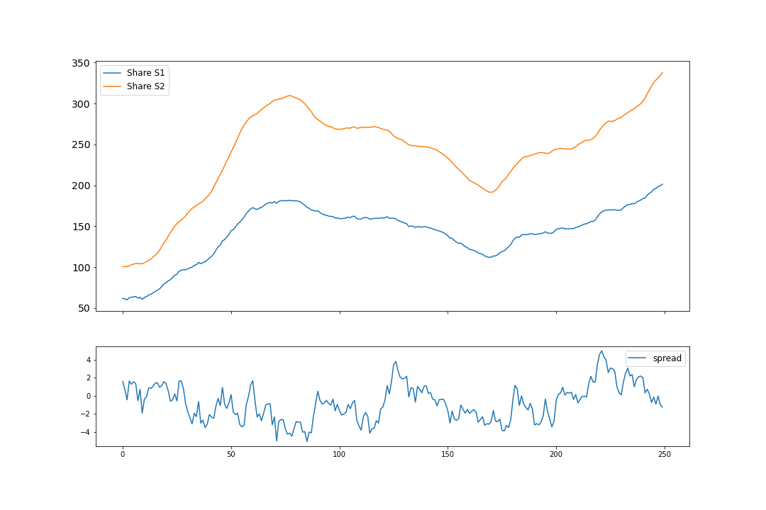
An example showcasing the cointegration simulation result. The parameters used are as follows.

\begin{eqnarray} \phi_1 & = & 0.95 \\ c_1 & = & 1.5 \\ \sigma_1 & = & 0.5 \\ \phi2 & = & 0.9 \\ c_2 & = & 0.05 \\ \sigma_2 & = & 1.0 \\ \beta & = & -0.6 \\ \end{eqnarray}

Implementation

This module allows simulation of cointegrated time series pairs.

class CointegrationSimulation(ts_num: int, ts_length: int)

This is a class that can be used to simulate cointegrated price series pairs.

The class will generate a price first-order difference time series defined by an AR(1) process, a cointegration error series defined by an AR(1) process, and calculate the other price series based on the cointegration equation.

__init__(ts_num: int, ts_length: int)

Initialize the simulation class.

Specify the number of time series to be simulated and define the length of each time series. Generate a default parameter set with the initialize_params method.

Parameters:

• ts_num – (int) Number of time series to simulate.

• ts_length – (int) Length of each time series to simulate.

get_coint_params() → dict

Getter for cointegration error simulation parameters.

Returns:

coint_params: (dict) Necessary parameters for cointegration error simulation.

get_price_params() → dict

Getter for price simulation parameters.

Returns:

price_params: (dict) Necessary parameters for share S2 price simulation.

static initialize_params() → Tuple[dict, dict]

Initialize the default parameters for the first-order difference of share S2 price series and cointegration error.

Returns:

(dict, dict) Necessary parameters for share S2 price simulation; necessary parameters for cointegration error simulation.

load_params(params: dict, target: str = 'price')

Setter for simulation parameters.

Change the entire parameter sets by loading the dictionary.

Parameters:

• params – (dict) Parameter dictionary.

• target – (str) Indicate which parameter to load. Possible values are “price” and “coint”.

plot_coint_series(series_x: array, series_y: array, coint_error: array, figw: float = 15.0, figh: float = 10.0) → Figure

Plot the simulated cointegrated series.

Parameters:

• series_x – (np.array) Price series of share S1

• series_y – (np.array) price series of share S2

• coint_error – (np.array) Cointegration error.

• figw – (float) Figure width.

• figh – (float) Figure height.

Returns:

(plt.Figure) Figure with the simulated cointegrated series.

set_coint_params(param: str, value: float)

Setter for cointegration error simulation parameters.

Change one specific parameter to a designated value. Possible parameters are [“ar_coeff”, “white_noise_var”, “constant_trend”, “beta”].

Parameters:

• param – (str) Parameter dictionary key.

• value – (float) Parameter value.

set_price_params(param: str, value: float)

Setter for price simulation parameters.

Change one specific parameter to a designated value. Possible parameters are [“ar_coeff”, “white_noise_var”, “constant_trend”].

Parameters:

• param – (str) Parameter dictionary key.

• value – (float) Parameter value.

simulate_ar(params: dict, burn_in: int = 50, use_statsmodels: bool = True) → array

Simulate an AR(1) process without using the statsmodels package. The AR(1) process is defined as the following recurrence relation.

\[y_t = \mu + \phi y_{t-1} + e_t, \quad e_t \sim N(0, \sigma^2) \qquad \mathrm{i.i.d}\]

Parameters:

• params – (dict) A parameter dictionary containing AR(1) coefficient, constant trend, and white noise variance.

• burn_in – (int) The amount of data used to burn in the process.

• use_statsmodel – (bool) If True, use statsmodels; otherwise, directly calculate recurrence.

Returns:

(np.array) ts_num simulated series generated.

simulate_coint(initial_price: float, use_statsmodels: bool = False) → Tuple[array, array, array]

Generate cointegrated price series and cointegration error series.

Parameters:

• initial_price – (float) Starting price of share S2.

• use_statsmodels – (bool) Use statsmodels API or use raw method. If True, then statsmodels API will be used.

Returns:

(np.array, np.array, np.array) Price series of share S1, price series of share S2, and cointegration error.

verify_ar(price_matrix: array) → Tuple[float, float | None]

Test function to confirm that the simulated price series is an AR(1) process.

Parameters:

price_matrix – (np.array) A matrix where each column is a hypothetical AR(1) process.

Returns:

(float, float) The mean AR(1) coefficient of the process; the standard deviation of AR(1) coefficient of the process.

verify_coint(price_series_x: array, price_series_y: array, x_name: str = 'Share S1', y_name: str = 'Share S2') → Tuple[float, float | None]

Use the Engle-Granger test to verify if the simulated series are cointegrated.

Parameters:

• price_series_x – (np.array) A matrix where each column is a simulated price series of share S1.

• price_series_y – (np.array) A matrix where each column is a simulated price series of share S2.

• x_name – (str) Column name for share S1 column of Engle-Granger input dataframe.

• y_name – (str) Column name for share S2 column of Engle-Granger input dataframe.

Returns:

(float, float) Mean of hedge ratio; standard deviation of hedge ratio.

Example

# Importing packages
from arbitragelab.cointegration_approach.coint_sim import CointegrationSimulation

# Generate 50 cointegrated time series, each of which has 250 data points
coint_simulator = CointegrationSimulation(50, 250)

# Setup the parameters for the AR(1) processes and cointegration coefficient, beta
price_params = {
"ar_coeff": 0.95,
"white_noise_var": 0.5,
"constant_trend": 1.5}

coint_params = {
    "ar_coeff": 0.9,
    "white_noise_var": 1.,
    "constant_trend": 0.05,
    "beta": -0.6}

coint_simulator.load_params(price_params, target='price')
coint_simulator.load_params(coint_params, target='coint')

# Perform simulation
s1_series, s2_series, coint_errors = coint_simulator.simulate_coint(initial_price=100.,
                                                                    use_statsmodels=True)

# Verify if the simulated series are cointegrated and the cointegration coefficient is equal to beta
beta_mean, beta_std = coint_simulator.verify_coint(s1_series, s2_series)

# Plot an example of the simulated series and their corresponding cointegration error
coint_sim_fig = coint_simulator.plot_coint_series(s1_series[:, 0], s2_series[:, 0],
                                                  coint_errors[:, 0])

Research Notebooks

• Minimum Profit Optimization

Download Notebook Download Sample Data

Research Article

Read our article I on the topic Read our article II on the topic

Presentation Slides

References

• Lin, Y.-X., McCrae, M., and Gulati, C., 2006. Loss protection in pairs trading through minimum profit bounds: a cointegration approach