Note

The following implementations and documentation closely follow the below work:

Mudchanatongsuk, S., Primbs, J.A. and Wong, W., 2008, June. Optimal pairs trading: A stochastic control approach.

OU Model Mudchanatongsuk

Introduction

In the paper corresponding to this module, the authors implement a stochastic control-based approach to the problem of pairs trading. The paper models the log-relationship between a pair of stock prices as an Ornstein-Uhlenbeck process and use this to formulate a portfolio optimization based stochastic control problem. This problem is constructed in such a way that one may either trade based on the spread (by buying and selling equal amounts of the stocks in the pair) or place money in a risk-free asset. Then the optimal solution to this control problem is obtained in closed form via the corresponding Hamilton-Jacobi-Bellman equation under a power utility on terminal wealth.

Modelling

Note

In this module and the corresponding paper,

\(k\) denotes the rate of mean reversion of the spread, \(\theta\) denotes the long run mean and, \(\eta\) denotes the standard deviation of the spread.

Let \(A(t)\) and \(B(t)\) denote respectively the prices of the pair of stocks \(A\) and \(B\) at time \(t\). The authors assume that stock \(B\) follows a geometric Brownian motion,

\[d B(t)=\mu B(t) d t+\sigma B(t) d Z(t)\]

where \(\mu\) is the drift, \(\sigma\) is the volatility, and \(Z(t)\) is a standard Brownian motion.

Let \(X(t)\) denote the spread of the two stocks at time \(t\), defined as

\[X(t) = \ln(A(t)) − \ln(B(t))\]

The authors assume that the spread follows an Ornstein-Uhlenbeck process

\[d X(t)=k(\theta-X(t)) d t+\eta d W(t)\]

where \(k\) is the rate of reversion, \(\eta\) is the standard deviation and \(\theta\) is the long-term equilibrium level to which the spread reverts.

\(\rho\) denotes the instantaneous correlation coefficient between \(Z(t)\) and \(W(t)\).

Let \(V(t)\) be the value of a self-financing pairs-trading portfolio and let \(h(t)\) and \(-h(t)\) denote respectively the portfolio weights for stocks \(A\) and \(B\) at time \(t\).

The wealth dynamics of the portfolio value is given by,

\[d V(t)= V(t)\left\{\left[h(t)\left(k(\theta-X(t))+\frac{1}{2} \eta^{2}+\rho \sigma \eta\right)+ r\right] d t+\eta d W(t)\right\}\]

Given below is the formulation of the portfolio optimization pair-trading problem as a stochastic optimal control problem. The authors assume that an investor’s preference can be represented by the utility function \(U(x) = \frac{1}{\gamma} x^\gamma\) with \(x ≥ 0\) and \(\gamma < 1\). In this formulation, our objective is to maximize expected utility at the final time \(T\). Thus, the authors seek to solve

\[\begin{split}\begin{aligned} \sup _{h(t)} \quad & E\left[\frac{1}{\gamma}(V(T))^{\gamma}\right] \\[0.8em] \text { subject to: } \quad & V(0)=v_{0}, \quad X(0)=x_{0} \\[0.5em] d X(t)=& k(\theta-X(t)) d t+\eta d W(t) \\ d V(t)=& V(t)((h(t)(k(\theta-X(t))+\frac{1}{2} \eta^{2}\\ &+\rho \sigma \eta)+r) d t+\eta d W(t)) \end{aligned}\end{split}\]

Finally, the optimal weights are given by,

\[h^{*}(t, x)=\frac{1}{1-\gamma}\left[\beta(t)+2 x \alpha(t)-\frac{k(x-\theta)}{\eta^{2}}+ \frac{\rho \sigma}{\eta}+\frac{1}{2}\right]\]

How to use this submodule

This submodule contains three public methods. One for estimating the parameters of the model using training data, and the second method is for calculating the final optimal portfolio weights using evaluation data.

Step 1: Model fitting

We input the training data to the fit method which calculates the spread and the estimators of the parameters of the model.

Implementation

Module implements the optimal pairs trading strategy using Stochastic Control Approach.

This module is a realization of the methodology in the following paper:

Mudchanatongsuk, S., Primbs, J.A. and Wong, W., 2008, June. Optimal pairs trading: A stochastic control approach.

class OUModelMudchanatongsuk

This class implements a stochastic control approach to the problem of pairs trading.

We model the log-relationship between a pair of stock prices as an OrnsteinUhlenbeck process, and use this to formulate a portfolio optimization based stochastic control problem. We are able to obtain the optimal solution to this control problem in closed form via the corresponding Hamilton-Jacobi-Bellman equation. This closed form solution is calculated under a power utility on terminal wealth. The parameters in the model are calculated using closed form maximum-likelihood estimation formulas.

__init__(): Initializes the parameters of the module.

OUModelMudchanatongsuk.fit(prices: DataFrame)

This method uses inputted training data to calculate the spread and estimate the parameters of the corresponding OU process.

The spread construction implementation follows Section II A in Mudchanatongsuk (2008).

Parameters:: prices – (pd.DataFrame) Contains price series of both stocks in spread.

Note

Although the paper provides closed form solutions for parameter estimation, this module uses log-likelihood maximization to estimate the parameters as we found the closed form solutions provided to be unstable.

Tip

To view the estimated model parameters from training data, call the describe function.

OUModelMudchanatongsuk.describe() → Series

Method returns values of instance attributes calculated from training data.

Returns:: (pd.Series) series describing parameter values.

Step 2: Getting the Optimal Portfolio Weights

In this step we input the evaluation data and specify the utility function parameter \(\gamma\).

Warning

As noted in the paper, please make sure the value of gamma is less than 1.

Implementation

OUModelMudchanatongsuk.optimal_portfolio_weights(prices: DataFrame, gamma: float = -100) → array

This method calculates the final optimal portfolio weights for the calculated spread.

The calculation of weights follows Section III in Mudchanatongsuk (2008), specifically equation 28.

Parameters:

prices – (pd.DataFrame) Contains price series of both stocks in spread.
gamma – (float) Parameter of utility function (gamma < 1).

Returns:

(np.array) Optimal weights array.

Tip

The spread_calc method can be used to calculate the spread on the test data.

OUModelMudchanatongsuk.spread_calc(prices: DataFrame) → tuple

This method calculates the spread on test data.

Parameters:: prices – (pd.DataFrame) Contains price series of both stocks in spread.
Returns:: (tuple) Consists of time remaining array and spread numpy array.

Example

We use GLD and GDX tickers from Yahoo Finance as the dataset for this example.

import yfinance as yf

data1 =  yf.download("GLD GDX", start="2012-03-25", end="2016-01-09")
data2 =  yf.download("GLD GDX", start="2016-02-21", end="2020-08-15")

data_train_dataframe = data1["Adj Close"][["GLD", "GDX"]]
data_test_dataframe = data2["Adj Close"][["GLD", "GDX"]]

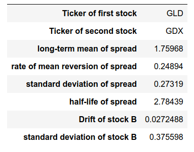
In the following code block, we are initializing the class and firstly, we use the fit method to generate the parameters of the model. Then, we call describe to view the estimated parameters. Finally, we use the out-of-sample test data to calculate the optimal portfolio weights using the fitted model.

from arbitragelab.stochastic_control_approach.ou_model_mudchanatongsuk import OUModelMudchanatongsuk

sc = OUModelMudchanatongsuk()

sc.fit(data_train_dataframe)

print(sc.describe())

plt.plot(sc.optimal_portfolio_weights(data_test_dataframe))
plt.show()

Research Notebook

The following research notebook can be used to better understand the approach described above.

Optimal Pairs Trading A Stochastic Control Approach

Research Article

Presentation Slides

References

Mudchanatongsuk, S., Primbs, J.A. and Wong, W., 2008, June. Optimal pairs trading: A stochastic control approach.