Cointegration Rules Spread Selection
The rules selection flow diagram from A Machine Learning based Pairs Trading Investment Strategy. by Simão Moraes Sarmento and Nuno Horta.
The rules that each spread needs to pass are:
The spread’s constituents are cointegrated. Literature suggests cointegration performs better than minimum distance and correlation approaches
The spread’s spread Hurst exponent reveals a mean-reverting character. Extra layer of validation.
The spread’s spread diverges and converges within convenient periods.
The spread’s spread reverts to the mean with enough frequency.
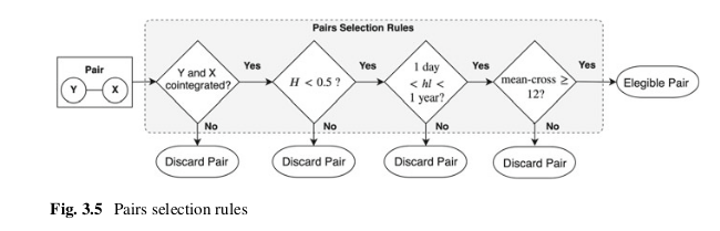
To test for cointegration, the framework proposes the application of the Engle-Granger test, due to its simplicity. One critic Armstrong (2001) points at the Engle-Granger test sensitivity to the ordering of variables. It is a possibility that one of the relationships will be cointegrated, while the other will not. This is troublesome because we would expect that if the variables are truly cointegrated the two equations will yield the same conclusion.
To mitigate this issue, the original paper proposes that the Engle-Granger test is run for the two possible selections of the dependent variable and that the combination that generated the lowest t-statistic is selected. Further work in Hoel (2013) adds on, “the unsymmetrical coefficients imply that a hedge of long / short is not the opposite of long / short , i.e. the hedge ratios are inconsistent”.
A better solution is proposed and implemented, based on Gregory et al. (2011) to use orthogonal regression – also referred to as Total Least Squares (TLS) – in which the residuals of both dependent and independent variables are taken into account. That way, we incorporate the volatility of both legs of the spread when estimating the relationship so that hedge ratios are consistent, and thus the cointegration estimates will be unaffected by the ordering of variables.
Hudson & Thames research team has also found out that optimal (in terms of cointegration tests statistics) hedge ratios are obtained by minimizng spread’s half-life of mean-reversion. Alongside this hedge ration calculation method, there is a wide variety of algorithms to choose from: TLS, OLS, Johansen Test Eigenvector, Box-Tiao Canonical Decomposition, Minimum Half-Life, Minimum ADF Test T-statistic Value.
Note
More information about the hedge ratio methods and their use can be found in the Hedge Ratio Calculations section of the documentation.
Secondly, an additional validation step is also implemented to provide more confidence in the mean-reversion character of the pairs’ spread. The condition imposed is that the Hurst exponent associated with the spread of a given pair is enforced to be smaller than 0.5, assuring the process leans towards mean-reversion.
In third place, the pair’s spread movement is constrained using the half-life of the mean-reverting process. In the framework paper the strategy built on top of the selection framework is based on the medium term price movements, so for this reason the spreads that either have very short (< 1 day) or very long mean-reversion (> 365 days) periods were not suitable.
Lastly, we enforce that every spread crosses its mean at least once per month, to provide enough liquidity and thus providing enough opportunities to exit a position.
Note
In practice to calculate the spread of the pairs supplied by this module, it is important to also consider the hedge ratio as follows:
\(S = leg1 - (hedgeratio_2) * leg2 - (hedgeratio_3) * leg3 - .....\)
Warning
The pairs selection function is very computationally heavy, so execution is going to be long and might slow down your system.
Note
The user may specify thresholds for each pair selector rule from the framework described above. For example, Engle-Granger test 99% threshold may seem too strict in pair selection which can be decreased to either 95% or 90%. On the other hand, the user may impose more strict thresholds on half life of mean reversion.
Note
H&T teams has extended pair selection rules to higher dimensions such that filtering rules can be applied to any spread, not only pairs. As a result, the module can be applied in statistical arbitrage applications.
Implementation
Examples
# Importing packages
import pandas as pd
import numpy as np
from arbitragelab.spread_selection.cointegration import CointegrationSpreadSelector

url = "https://raw.githubusercontent.com/hudson-and-thames/example-data/main/arbitrage_lab_data/sp100_prices.csv"
data = pd.read_csv(url, index_col=0, parse_dates=[0])
input_spreads = [('ABMD', 'AZO'), ('AES', 'BBY'), ('BKR', 'CE'), ('BKR', 'CE', 'AMZN')]
pairs_selector = CointegrationSpreadSelector(prices_df=data, baskets_to_filter=input_spreads)
filtered_spreads = pairs_selector.select_spreads(hedge_ratio_calculation='TLS',
                                                 adf_cutoff_threshold=0.9,
                                                 hurst_exp_threshold=0.55,
                                                 min_crossover_threshold=0,
                                                 min_half_life=20)

# Statistics logs data frame.
logs = pairs_selector.selection_logs.copy()

# A user may also specify own constructed spread to be tested.
spread = pd.read_csv('spread.csv', index_col=0, parse_dates=[0])
pairs_selector = CointegrationSpreadSelector(prices_df=None, baskets_to_filter=None)
# Using log_info=True to save stats.
stats = pairs_selector.generate_spread_statistics(spread, log_info=True)
print(pairs_selector.selection_logs)
print(stats)
filtered_spreads = pairs_selector.apply_filtering_rules(adf_cutoff_threshold=0.99,
                                                        hurst_exp_threshold=0.5)
Research Notebooks
The following research notebook can be used to better understand the Cointegration Rules Spread Selection described above.