Note
The following implementations and documentation closely follow the work of Tim Leung: Tim Leung and Xin Li Optimal Mean reversion Trading: Mathematical Analysis and Practical Applications.
Trading Under the Cox-Ingersoll-Ross Model
Warning
Alongside with Leung’s research we are using \(\theta\) for mean and \(\mu\) for mean-reversion speed, while other sources e.g. Wikipedia, use \(\theta\) for mean reversion speed and \(\mu\) for mean.
Model fitting
Note
We are solving the optimal stopping problem for a mean-reverting portfolio that is constructed by holding \(\alpha = \frac{A}{S_0^{(1)}}\) of a risky asset \(S^{(1)}\) and shorting \(\beta = \frac{B}{S_0^{(2)}}\) of another risky asset \(S^{(2)}\), yielding a portfolio value:
Since in terms of mean-reversion we care only about the ratio between \(\alpha\) and \(\beta\), without the loss of generality we can set \(\alpha = const\) and A = $1, while varying \(\beta\) to find the optimal strategy \((\alpha,\beta^*)\)
We establish a Cox-Ingersoll-Ross process driven by the SDE:
\(\theta\) − long term mean level, all future trajectories of Y will evolve around a mean level 𝜃 in the long run.
\(\mu\) - speed of reversion, characterizes the velocity at which such trajectories will regroup around \(\theta\) in time.
\(\sigma\) - instantaneous volatility, measures instant by instant the amplitude of randomness entering the system. Higher values imply more randomness.
To fit the model to our data and find optimal parameters we define the average log-likelihood function as in Borodin and Salminen (2002):
Then, maximizing the log-likelihood function by applying maximum likelihood estimation(MLE) we are able to determine the parameters of the model and fit the observed portfolio prices to a CIR process. Let’s denote the maximized average log-likelihood by \(\hat{\ell}(\theta^*,\mu^*,\sigma^*)\). Then for every \(\alpha\) we choose \(\beta^*\), where:
Optimal Timing of Trades
To find the optimal timing of trades we have implemented two approaches - optimal stopping and optimal switching. The main difference between the two is the assumption about the number of trades in regards to which we are searching for the optimal timing of trades. In case of an optimal stopping problem, we assume that we want to search for such optimal levels that will maximize the output of a single entry-exit pair of trades. On the other hand, the optimal switching approach is aimed at maximizing the infinite amount of entry-exit trades, thus accounting for any number of consequent trades our investor might want to carry out.
Optimal stopping problem
Suppose the investor already has a position with a value process \((Y_t)_{t>0}\) that follows the CIR process. When the investor closes his position at the time \(\tau\) he receives the value \((Y_{\tau})\) and pays a constant transaction cost \(c_s \in \mathbb{R}\) To maximize the expected discounted value we need to solve the optimal stopping problem:
where \(T\) denotes the set of all possible stopping times and \(r > 0\) is our subjective constant discount rate. \(V^{\chi}(y)\) represents the expected liquidation value accounted with y.
Current price plus transaction cost constitute the cost of entering the trade and in combination with \(V^{\chi}(y)\) we can formalize the optimal entry problem:
with
To sum up this problem, we, as an investor, want to maximize the expected difference between the current price of the position - \(Y_{\nu}\) and its’ expected liquidation value \(V^{\chi}(Y_{\nu})\) minus transaction cost \(c_b\)
Note
Following part of the chapter presents the analytical solution for the optimal stopping problem, both the default version and the version with the inclusion of the stop-loss level.
To solve this problem we denote the CIR process infinitesimal generator:
and recall the classical solution of the differential equation
Then we are able to formulate the following theorems (proven in Optimal Mean reversion Trading: Mathematical Analysis and Practical Applications by Tim Leung and Xin Li) to provide the solutions to the following problems:
Theorem 4.2 (p.85):
The optimal liquidation problem admits the solution:
The optimal liquidation level \(b^{\chi*}\) is found from the equation:
Corresponding optimal liquidation time is given by
Theorem 4.4 (p.86):
The optimal entry timing problem admits the solution:
The optimal entry level \(d^{\chi*}\) is found from the equation:
Where “\(\hat{\ }\)” represents the use of transaction cost and discount rate of entering.
Optimal switching problem
To find the optimal levels, first, two critical constants have to be denoted:
Theorem 4.7 (p.56):
Under the optimal switching approach it is optimal to re-enter the market if and only if all of the following conditions hold true:
If \(y_b>0\)
The following inequality must hold true:
In case any of the conditions are not met - re-entering the market is deemed not optimal. It would be advised to exit at the optimal liquidation price without re-entering, or not enter the position at all. The difference between the options depends on whether the investor had already entered the market beforehand, or did he or she start with a zero position.
How to use this submodule
This module provides you tools for obtaining the solutions to optimal stopping and optimal switching problems for the CIR model.
Step 1: Model fitting
During the module fitting stage, we need to use fit function to fit the CIR model to our training data. The data provided
should consist of a log-price of an already created mean-reverting portfolio.
Implementation
Tip
To retrain the model just use one of the functions fit_to_portfolio or fit_to_assets.
You have a choice either to use the new dataset or to change the training time interval of your currently
used dataset.
Step 2: Determining the optimal entry and exit values
To get the optimal liquidation or entry level for your data we need to call one of the functions mentioned below. They present the solutions to the equations established during the theoretical part. To choose whether to account for the stop-loss level or not choose the respective set of functions.
Implementation
\(b^{\chi*}\): - optimal level of liquidation:
\(d^{\chi*}\) - optimal level of entry, accounting for preferred stop-loss level:
Tip
General rule for the use of the optimal levels:
If not bought, buy the portfolio as soon as portfolio price reaches the optimal entry level (enters the interval).
If bought, liquidate the position as soon as portfolio price reaches the optimal liquidation level.
Step 3: Determining the optimal switching entry and exit values
To get the optimal switching values we need to use the optimal_switching_levels function that either returns
the interval of optimal switching prices or an optimal liquidation level if it is deemed not optimal to re-enter the market.
Implementation
Step 4: (Optional) Plot the optimal levels on your data
Additionally, you have the ability to plot your optimal levels for default problem and optimal switching onto your out-of-sample data. You have a choice whether you want the optimal switching levels displayed or not.
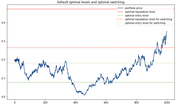
An exemplary output of the cir_plot_levels function.
Implementation
Tip
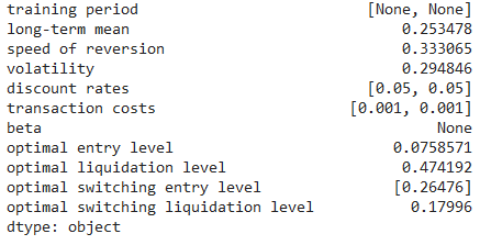
To view all the model stats, including the optimal levels call the cir_description function.
Example
import numpy as np
from arbitragelab.optimal_mean_reversion import CoxIngersollRoss

example = CoxIngersollRoss()

# We establish our training sample
delta_t = 1/252
np.random.seed(30)
cir_example =  example.cir_model_simulation(n=1000, theta_given=0.2, mu_given=0.2,
                                            sigma_given=0.3, delta_t_given=delta_t)
# Model fitting
example.fit(cir_example, data_frequency="D", discount_rate=0.05,
            transaction_cost=[0.001, 0.001])

# You can separately solve optimal stopping
# and optimal switching problems

# Solving the optimal stopping problem
b = example.optimal_liquidation_level()

d = example.optimal_entry_level()

# Solving the optimal switching problem
d_switch, b_switch = example.optimal_switching_levels()

# You can display the results using the plot
fig = example.cir_plot_levels(cir_example, switching=True)

# Or you can view the model statistics
example.cir_description(switching=True)
Research Notebook
The following research notebook can be used to better understand the concepts of trading under the Cox-Ingersoll-Ross Model.