Note

The following documentation closely follows a paper by Marco Avellaneda and Jeong-Hyun Lee: Statistical Arbitrage in the U.S. Equities Market.

PCA Approach

Introduction

This module shows how the Principal Component Analysis can be used to create mean-reverting portfolios and generate trading signals. It’s done by considering residuals or idiosyncratic components of returns and modeling them as mean-reverting processes.

The original paper presents the following description:

The returns for different stocks are denoted as \(\{ R_{i} \}^{N}_{i=1}\). The \(F\) represents the return of a “market portfolio” over the same period. For each stock in the universe:

\[R_{i} = \beta_{i} F + \widetilde{R_{i}}\]

which is a regression, decomposing stock returns into a systematic component \(\beta_{i} F\) and an (uncorrelated) idiosyncratic component \(\widetilde{R_{i}}\).

This can also be extended to a multi-factor model with \(m\) systematic factors:

\[R_{i} = \sum^{m}_{j=1} \beta_{ij} F_{j} + \widetilde{R_{i}}\]

A trading portfolio is a market-neutral one if the amounts \(\{ Q_{i} \}^{N}_{i=1}\) invested in each of the stocks are such that:

\[\bar{\beta}_{j} = \sum^{N}_{i=1} \beta_{ij} Q_{i} = 0, j = 1, 2,, ..., m.\]

where \(\bar{\beta}_{j}\) correspond to the portfolio betas - projections of the portfolio returns on different factors.

As derived in the original paper,

\[\sum^{N}_{i=1} Q_{i} R_{i} = \sum^{N}_{i=1} Q_{i} \widetilde{R_{i}}\]

So, a market-neutral portfolio is only affected by idiosyncratic returns.

PCA Approach

This approach was originally proposed by Jolliffe (2002). It is using a historical share price data on a cross-section of \(N\) stocks going back \(M\) days in history. The stocks return data on a date \(t_{0}\) going back \(M + 1\) days can be represented as a matrix:

\[R_{ik} = \frac{S_{i(t_{0} - (k - 1) \Delta t)} - S_{i(t_{0} - k \Delta t)}}{S_{i(t_{0} - k \Delta t)}}; k = 1, ..., M; i = 1, ..., N.\]

where \(S_{it}\) is the price of stock \(i\) at time \(t\) adjusted for dividends. For daily observations \(\Delta t = 1 / 252\).

Returns are standardized, as some assets may have greater volatility than others:

\[Y_{ik} = \frac{R_{ik} - \bar{R_{i}}}{\bar{\sigma_{i}}}\]

where

\[\bar{R_{i}} = \frac{1}{M} \sum^{M}_{k=1}R_{ik}\]

and

\[\bar{\sigma_{i}}^{2} = \frac{1}{M-1} \sum^{M}_{k=1} (R_{ik} - \bar{R_{i}})^{2}\]

And the empirical correlation matrix is defined by

\[\rho_{ij} = \frac{1}{M-1} \sum^{M}_{k=1} Y_{ik} Y_{jk}\]

Note

It’s important to standardize data before inputting it to PCA, as the PCA seeks to maximize the variance of each component. Using unstandardized input data will result in worse results. The get_signals() function in this module automatically standardizes input returns before feeding them to PCA.

The original paper mentions that picking long estimation windows for the correlation matrix (\(M \gg N\), \(M\) is the estimation window, \(N\) is the number of assets in a portfolio) don’t make sense because they take into account the distant past which is economically irrelevant. The estimation windows used by the authors is fixed at 1 year (252 trading days) prior to the trading date.

The eigenvalues of the correlation matrix are ranked in the decreasing order:

\[N \ge \lambda_{1} \ge \lambda_{2} \ge \lambda_{3} \ge ... \ge \lambda_{N} \ge 0.\]

And the corresponding eigenvectors:

\[v^{(j)} = ( v^{(j)}_{1}, ..., v^{(j)}_{N} ); j = 1, ..., N.\]

Now, for each index \(j\) we consider a corresponding “eigen portfolio”, in which we invest the respective amounts invested in each of the stocks as:

\[Q^{(j)}_{i} = \frac{v^{(j)}_{i}}{\bar{\sigma_{i}}}\]

And the eigen portfolio returns are:

\[F_{jk} = \sum^{N}_{i=1} \frac{v^{(j)}_{i}}{\bar{\sigma_{i}}} R_{ik}; j = 1, 2, ..., m.\]

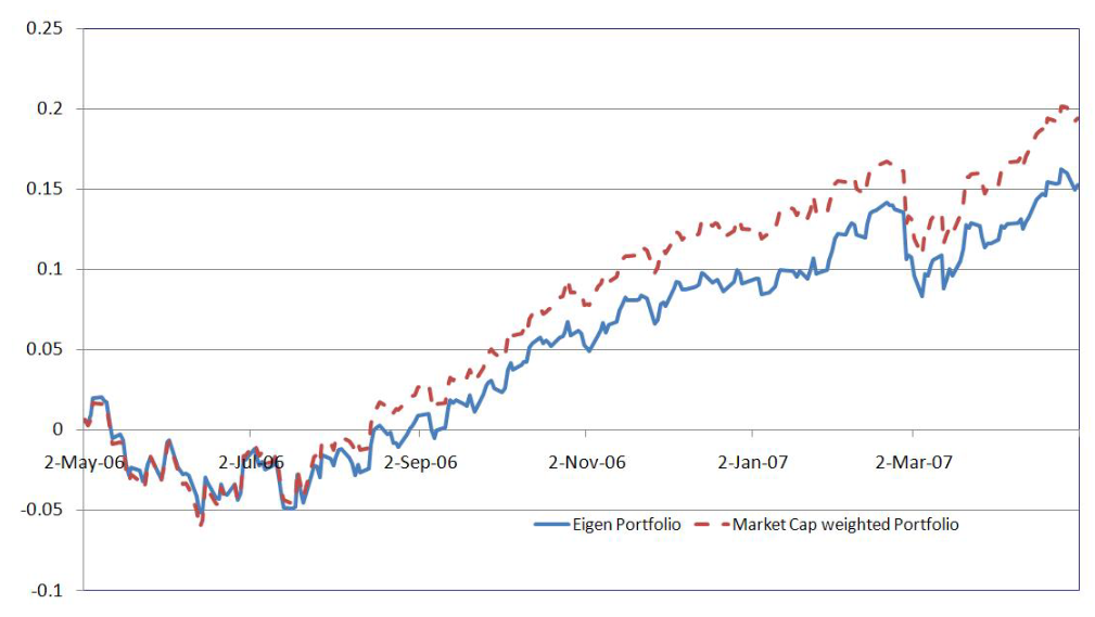
Performance of a portfolio composed using the PCA approach in comparison to the market cap portfolio. An example from Statistical Arbitrage in the U.S. Equities Market. by Marco Avellaneda and Jeong-Hyun Lee.

In a multi-factor model we assume that stock returns satisfy the system of stochastic differential equations:

\[\frac{dS_{i}(t)}{S_{i}(t)} = \alpha_{i} dt + \sum^{N}_{j=1} \beta_{ij} \frac{dI_{j}(t)}{I_{j}(t)} + dX_{i}(t),\]

where \(\beta_{ij}\) are the factor loadings.

The idiosyncratic component of the return with drift \(\alpha_{i}\) is:

\[d \widetilde{X_{i}}(t) = \alpha_{i} dt + d X_{i} (t).\]

Based on the previous descriptions, a model for \(X_{i}(t)\) is estimated as the Ornstein-Uhlenbeck process:

\[dX_{i}(t) = \kappa_{i} (m_{i} - X_{i}(t))dt + \sigma_{i} dW_{i}(t), \kappa_{i} > 0.\]

which is stationary and auto-regressive with lag 1.

Note

To find out more about the Ornstein-Uhlenbeck model and optimal trading under this model please check out our section on Trading Under the Ornstein-Uhlenbeck Model.

The parameters \(\alpha_{i}, \kappa_{i}, m_{i}, \sigma_{i}\) are specific for each stock. They are assumed to de facto vary slowly in relation to Brownian motion increments \(dW_{i}(t)\), in the chosen time-window. The authors of the paper were using a 60-day window to estimate the residual processes for each stock and assumed that these parameters were constant over the window.

However, the hypothesis of parameters being constant over the time-window is being accepted for stocks which mean reversion (the estimate of \(\kappa\)) is sufficiently high and is rejected for stocks with a slow speed of mean-reversion.

An investment in a market long-short portfolio is being constructed by going long $1 on the stock and short \(\beta_{ij}\) dollars on the \(j\) -th factor. Expected 1-day return of such portfolio is:

\[\alpha_{i} dt + \kappa_{i} (m_{i} - X_{i}(t))dt\]

The parameter \(\kappa_{i}\) is called the speed of mean-reversion. If \(\kappa \gg 1\) the stock reverts quickly to its means and the effect of drift is negligible. As we are assuming that the parameters of our model are constant, we are interested in stocks with fast mean-reversion, such that:

\[\frac{1}{\kappa_{i}} \ll T_{1}\]

where \(T_{1}\) is the estimation window to estimate residuals in years.

Implementation

class PCAStrategy(n_components: int = 15)

This strategy creates mean reverting portfolios using Principal Components Analysis. The idea of the strategy is to estimate PCA factors affecting the dynamics of assets in a portfolio. Thereafter, for each asset in a portfolio, we define OLS residuals by regressing asset returns on PCA factors. These residuals are used to calculate S-scores to generate trading signals and the regression coefficients are used to construct eigen portfolios for each asset. If the eigen portfolio shows good mean-reverting properties and the S-score deviates enough from its mean value, that eigen portfolio is being traded. The output trading signals of this strategy are weights for each asset in a portfolio at each given time. These weights are are a composition of all eigen portfolios that satisfy the required properties.

__init__(n_components: int = 15)

Initialize PCA StatArb Strategy.

The original paper suggests that the number of components would be chosen to explain at least 50% of the total variance in time. Authors also denote that for G8 economies, stock returns are explained by approximately 15 factors (or between 10 and 20 factors).

Parameters:

n_components – (int) Number of PCA principal components to use in order to build factors.

get_factorweights(matrix: DataFrame) → DataFrame

A function to calculate weights (scaled eigen vectors) to use for factor return calculation.

Weights are calculated from PCA components as:

Weight = Eigen vector / st.d.(R)

So the output is a dataframe containing the weight for each asset in a portfolio for each eigen vector.

Parameters:

matrix – (pd.DataFrame) Dataframe with index and columns containing asset returns.

Returns:

(pd.DataFrame) Weights (scaled PCA components) for each index from the matrix.

static get_sscores(residuals: DataFrame, k: float) → Series

A function to calculate S-scores for asset eigen portfolios given dataframes of residuals and a mean reversion speed threshold.

From residuals, a discrete version of the OU process is created for each asset eigen portfolio.

If the OU process of the asset shows a mean reversion speed above the given threshold k, it can be traded and the S-score is being calculated for it.

The output of this function is a dataframe with S-scores that are directly used to determine if the eigen portfolio of a given asset should be traded at this period.

In the original paper, it is advised to choose k being less than half of a window for residual estimation. If this window is 60 days, half of it is 30 days. So k > 252/30 = 8.4. (Assuming 252 trading days in a year)

Parameters:

• residuals – (pd.DataFrame) Dataframe with residuals after fitting returns to PCA factor returns.

• k – (float) Required speed of mean reversion to use the eigen portfolio in trading.

Returns:

(pd.Series) Series of S-scores for each asset for a given residual dataframe.

static standardize_data(matrix: ~pandas.core.frame.DataFrame) -> (<class 'pandas.core.frame.DataFrame'>, <class 'pandas.core.series.Series'>)

A function to standardize data (returns) that is being fed into the PCA.

The standardized returns (R)are calculated as:

R_standardized = (R - mean(R)) / st.d.(R)

Parameters:

matrix – (pd.DataFrame) DataFrame with returns that need to be standardized.

Returns:

(pd.DataFrame. pd.Series) a tuple with two elements: DataFrame with standardized returns and Series of standard deviations.

PCA Trading Strategy

The strategy implemented sets a default estimation window for the correlation matrix as 252 days, a window for residuals estimation of 60 days (\(T_{1} = 60/252\)) and the threshold for the mean reversion speed of an eigen portfolio for it to be traded so that the reversion time is less than \(1/2\) period (\(\kappa > 252/30 = 8.4\)).

For the process \(X_{i}(t)\) the equilibrium variance is defined as:

\[\sigma_{eq,i} = \frac{\sigma_{i}}{\sqrt{2 \kappa_{i}}}\]

And the following variable is defined:

\[s_{i} = \frac{X_{i}(t)-m_{i}}{\sigma_{eq,i}}\]

This variable is called the S-score. The S-score measures the distance to the equilibrium of the cointegrated residual in units standard deviations, i.e. how far away a given asset eigen portfolio is from the theoretical equilibrium value associated with the model.

Evolution of the S-score of JPM ( vs. XLF ) from January 2006 to December 2007. An example from Statistical Arbitrage in the U.S. Equities Market. by Marco Avellaneda and Jeong-Hyun Lee.

If the eigen portfolio shows a mean reversion speed above the set threshold (\(\kappa\)), the S-score based on the values from the residual estimation window is being calculated.

The trading signals are generated from the S-scores using the following rules:

• Open a long position if \(s_{i} < - \bar{s_{bo}}\)

• Close a long position if \(s_{i} < + \bar{s_{bc}}\)

• Open a short position if \(s_{i} > + \bar{s_{so}}\)

• Close a short position if \(s_{i} > - \bar{s_{sc}}\)

Opening a long position means buying $1 of the corresponding stock (of the asset eigen portfolio) and selling \(\beta_{i1}\) dollars of assets from the first scaled eigenvector (\(Q^{(1)}_{i}\)), \(\beta_{i2}\) from the second scaled eigenvector (\(Q^{(2)}_{i}\)) and so on.

Opening a short position, on the other hand, means selling $1 of the corresponding stock and buying respective beta values of stocks from scaled eigenvectors.

Authors of the paper, based on empirical analysis chose the following cutoffs. They were selected based on simulating strategies from 2000 to 2004 in the case of ETF factors:

• \(\bar{s_{bo}} = \bar{s_{so}} = 1.25\)

• \(\bar{s_{bc}} = 0.75\), \(\bar{s_{sc}} = 0.50\)

The rationale behind this strategy is that we open trades when the eigen portfolio shows good mean reversion speed and its S-score is far from the equilibrium, as we think that we detected an anomalous excursion of the co-integration residual. We expect most of the assets in our portfolio to be near equilibrium most of the time, so we are closing trades at values close to zero.

The signal generating function implemented in the ArbitrageLab package outputs target weights for each asset in our portfolio for each observation time - target weights here are the sum of weights of all eigen portfolios that show high mean reversion speed and have needed S-score value at a given time.

Implementation

class PCAStrategy(n_components: int = 15)

This strategy creates mean reverting portfolios using Principal Components Analysis. The idea of the strategy is to estimate PCA factors affecting the dynamics of assets in a portfolio. Thereafter, for each asset in a portfolio, we define OLS residuals by regressing asset returns on PCA factors. These residuals are used to calculate S-scores to generate trading signals and the regression coefficients are used to construct eigen portfolios for each asset. If the eigen portfolio shows good mean-reverting properties and the S-score deviates enough from its mean value, that eigen portfolio is being traded. The output trading signals of this strategy are weights for each asset in a portfolio at each given time. These weights are are a composition of all eigen portfolios that satisfy the required properties.

__init__(n_components: int = 15)

Initialize PCA StatArb Strategy.

The original paper suggests that the number of components would be chosen to explain at least 50% of the total variance in time. Authors also denote that for G8 economies, stock returns are explained by approximately 15 factors (or between 10 and 20 factors).

Parameters:

n_components – (int) Number of PCA principal components to use in order to build factors.

get_signals(matrix: DataFrame, k: float = 8.4, corr_window: int = 252, residual_window: int = 60, sbo: float = 1.25, sso: float = 1.25, ssc: float = 0.5, sbc: float = 0.75, size: float = 1) → DataFrame

A function to generate trading signals for given returns matrix with parameters.

First, the correlation matrix to get PCA components is calculated using a corr_window parameter. From this, we get weights to calculate PCA factor returns. These weights are being recalculated each time we generate (residual_window) number of signals.

It is expected that corr_window>residual_window. In the original paper, corr_window is set to 252 days and residual_window is set to 60 days. So with corr_window==252, the first 252 observation will be used for estimation and the first signal will be generated for the 253rd observation.

Next, we pick the last (residual_window) observations to compute PCA factor returns and fit them to residual_window observations to get residuals and regression coefficients.

Based on the residuals the S-scores are being calculated. These S-scores are calculated as:

s_i = (X_i(t) - m_i) / sigma_i

Where X_i(t) is the OU process generated from the residuals, m_i and sigma_i are the calculated properties of this process.

The S-score is being calculated only for eigen portfolios that show mean reversion speed above the given threshold k.

In the original paper, it is advised to choose k being less than half of a window for residual estimation. If this window is 60 days, half of it is 30 days. So k > 252/30 = 8.4. (Assuming 252 trading days in a year)

So, we can have mean-reverting eigen portfolios for each asset in our portfolio. But this portfolio is worth investing in only if it shows good mean reversion speed and the S-score has deviated enough from its mean value. Based on this logic we pick promising eigen portfolios and invest in them. The trading signals we get are the target weights for each of the assets in our portfolio at any given time.

Trading rules to enter a mean-reverting portfolio based on the S-score are:

Enter a long position if s-score < −sbo Close a long position if s-score > −ssc Enter a short position if s-score > +sso Close a short position if s-score < +sbc

The authors empirically chose the optimal values for the above parameters based on stock prices for years 2000-2004 as: sbo = sso = 1.25; sbc = 0.75; ssc = 0.5.

Opening a long position on an eigne portfolio means buying one dollar of the corresponding asset and selling beta_i1 dollars of weights of other assets from component1, beta_i2 dollars of weights of other assets from component2 and so on. Opening a short position means selling the corresponding asset and buying betas of other assets.

Parameters:

• matrix – (pd.DataFrame) Dataframe with returns for assets.

• k – (float) Required speed of mean reversion to use the eigen portfolio in trading.

• corr_window – (int) Look-back window used for correlation matrix estimation.

• residual_window – (int) Look-back window used for residuals calculation.

• sbo – (float) Parameter for signal generation for the S-score.

• sso – (float) Parameter for signal generation for the S-score.

• ssc – (float) Parameter for signal generation for the S-score.

• sbc – (float) Parameter for signal generation for the S-score.

• size – (float) Number of units invested in assets when opening trades. So when opening a long position, buying (size) units of stock and selling (size) * betas units of other stocks.

Returns:

(pd.DataFrame) DataFrame with target weights for each asset at every observation. It is being calculated as a combination of all eigen portfolios that are satisfying the mean reversion speed requirement and S-score values.

static get_sscores(residuals: DataFrame, k: float) → Series

A function to calculate S-scores for asset eigen portfolios given dataframes of residuals and a mean reversion speed threshold.

From residuals, a discrete version of the OU process is created for each asset eigen portfolio.

If the OU process of the asset shows a mean reversion speed above the given threshold k, it can be traded and the S-score is being calculated for it.

The output of this function is a dataframe with S-scores that are directly used to determine if the eigen portfolio of a given asset should be traded at this period.

In the original paper, it is advised to choose k being less than half of a window for residual estimation. If this window is 60 days, half of it is 30 days. So k > 252/30 = 8.4. (Assuming 252 trading days in a year)

Parameters:

• residuals – (pd.DataFrame) Dataframe with residuals after fitting returns to PCA factor returns.

• k – (float) Required speed of mean reversion to use the eigen portfolio in trading.

Returns:

(pd.Series) Series of S-scores for each asset for a given residual dataframe.

Examples

# Importing packages
import pandas as pd
import numpy as np
from arbitragelab.other_approaches.pca_approach import PCAStrategy

# Getting the dataframe with time series of asset returns
data = pd.read_csv('X_FILE_PATH.csv', index_col=0, parse_dates = [0])

# The PCA Strategy class that contains all needed methods
pca_strategy = PCAStrategy()

# Simply applying the PCAStrategy with standard parameters
target_weights = pca_strategy.get_signals(data, k=8.4, corr_window=252,
                                          residual_window=60, sbo=1.25,
                                          sso=1.25, ssc=0.5, sbc=0.75,
                                          size=1)

# Or we can do individual actions from the PCA approach
# Standardizing the dataset
data_standardized, data_std = pca_strategy.standardize_data(data)

# Getting factor weights using the first 252 observations
data_252days = data[:252]
factorweights = pca_strategy.get_factorweights(data_252days)

# Calculating factor returns for a 60-day window from our factor weights
data_60days = data[(252-60):252]
factorret = pd.DataFrame(np.dot(data_60days, factorweights.transpose()),
                         index=data_60days.index)

# Calculating residuals for a set 60-day window
residual, coefficient = pca_strategy.get_residuals(data_60days, factorret)

# Calculating S-scores for each eigen portfolio for a set 60-day window
s_scores = pca_strategy.get_sscores(residual, k=8)

Research Notebooks

The following research notebook can be used to better understand the PCA approach described above.

• PCA Approach

Download Notebook Download Sample Data

Presentation Slides

References

• Avellaneda, M. and Lee, J.H., 2010. Statistical arbitrage in the US equities market. Quantitative Finance, 10(7), pp.761-782.

• Jolliffe, I. T., Principal Components Analysis, Springer Series in Statistics, Springer-Verlag, Heidelberg, 2002.