Note

The following implementations and documentation closely follow the below work:

Jurek, J.W. and Yang, H., 2007, April. Dynamic portfolio selection in arbitrage.

OU Model Jurek

Introduction

In the paper corresponding to this module, the authors derive the optimal dynamic strategy for arbitrageurs with a finite horizon and non-myopic preferences facing a mean-reverting arbitrage opportunity (e.g. an equity pairs trade).

The law of one price asserts that - in a frictionless market - securities with identical payoffs must trade at identical prices. If this were not the case, arbitrageurs could generate a riskless profit by supplying (demanding) the expensive (cheap) asset until the mispricing was eliminated. Of course, real world markets are not frictionless, and the prices of securities with identical payoffs may significantly diverge for extended periods of time. Arbitrageurs can earn potentially attractive profits by taking offsetting positions in these relatively mispriced securities, but a worsening of the mispricing can result in sizable capital losses.

Unlike textbook arbitrages, which generate riskless profits and require no capital commitments, exploiting real-world mispricings requires the assumption of some combination of horizon and divergence risk. These two risks represent the uncertainty about whether the mispricing will converge before the positions must be closed (or profits reported) and the possibility of a worsening in the mispricing prior to its elimination.

While a complete treatment of optimal arbitrage and price formation requires a general equilibrium framework, this paper takes on the more modest goal of examining the arbitrageur’s strategy in partial equilibrium.

Modelling

Note

In this module and the corresponding paper,

\(\kappa\) denotes the rate of mean reversion of the spread, \(\mu\) denotes the long run mean and, \(\sigma\) denotes the standard deviation of the spread.

To capture the presence of horizon and divergence risk, the authors model the dynamics of the mispricing using a mean-reverting stochastic process. Under this process, although the mispricing is guaranteed to be eliminated at some future date, the timing of convergence, as well as the maximum magnitude of the mispricing prior to convergence, are uncertain. With this assumption, the authors are able to derive the arbitrageur’s optimal dynamic portfolio policy for a set of general, non-myopic preference specifications, including CRRA utility defined over wealth at a finite horizon and Epstein-Zin utility defined over intermediate cash flows (e.g. fees). This allows us to analytically examine the role of intertemporal hedging demands in arbitrage activities and represents a novel contribution relative to the commonly assumed log utility specification, under which hedging demands are absent.

It was observed that, in the presence of horizon and divergence risk, there is a critical level of the mispricing beyond which further divergence in the mispricing precipitates a reduction in the allocation. Although a divergence in the mispricing results in an improvement in the instantaneous investment opportunity set and should induce added participation by rational arbitrageurs, this effect can be more than offset by the combination of the loss in wealth and the nearing of the evaluation date, which reduce the arbitrageur’s effective risk-bearing capacity. The complex tradeoff between these two effects leads to the creation of a time-varying boundary, outside of which continued divergence of the mispricing induces rational arbitrageurs to cut their losses and decrease their allocations to the mispricing.

The central assumption of our model is that the arbitrage opportunity is described by an Ornstein-Uhlenbeck process (henceforth OU). The OU process captures the two key features of a real-world mispricing: the convergence times are uncertain and the mispricing can diverge arbitrarily far from its mean prior to convergence.

The optimal trading strategies derived are self-financing and can be interpreted as the optimal trading rules for a fund which is not subject to withdrawals but also cannot raise additional assets (i.e. a closed-end fund). The dynamics of the optimal allocation to the arbitrage opportunity are driven by two factors: the necessity of maintaining wealth (equity) above zero and the proximity of the arbitrageur’s terminal evaluation date, which affects his appetite for risk.

Investor Preferences

The authors considered two alternative preferences structures for the arbitrageur in our continuous-time model. In the first, the authors assumed that the agent has constant relative risk aversion and maximizes the discounted utility of terminal wealth. The arbitrageur’s value function at time \(t\) - denoted by \(V_t\) - takes the form:

\[V_{t}=\sup E_{t}\left[e^{-\beta(T-t)} \frac{W_{T}^{1-\gamma}}{1-\gamma}\right]\]

The second preference structure they considered is the recursive utility of Epstein and Zin (1989, 1991), which allows the elasticity of intertemporal substitution and the coefficient of relative risk aversion to vary independently. Under this preference specification, the value function of the arbitrageur is given by:

\[V_{t}=\sup E_{t}\left[\int_{t}^{T} f\left(C_{s}, J_{s}\right) d s\right]\]

where \(f\left(C_{s}, J_{s}\right)\) is the normalized aggregator for the continuous-time Epstein-Zin utility function:

\[f\left(C_{t}, J_{t}\right)=\beta(1-\gamma) \cdot J_{t} \cdot\left[\log C_{t}-\frac{1}{1-\gamma} \log \left((1-\gamma) J_{t}\right)\right]\]

Here the authors considered the special case of a unit elasticity of intertemporal substitution (\(\psi = 1\)).

Here \(C_t\) denotes the instantaneous consumption (e.g. cash flow). \(\beta\) is the rate of time preference, and \(\gamma\) is the coefficient of relative risk aversion.

Note

In this paper, the choice of preference structures is driven by economic intuition regarding the incentives of real-life arbitrageurs. In particular, it can be assumed that the arbitrageur is a proprietary trading desk or delegated money manager with a fixed investment horizon. It seems likely that such investors would only be interested in the distribution of wealth at a finite horizon, e.g. at the end of the fiscal year, rather than the value of a long-dated consumption stream.

However, the decision to model arbitrageurs as finite-horizon CRRA investors neglects the role of management fees, which are often collected by arbitrageurs. To capture this feature, the authors also consider the Epstein-Zin model specialized to the case of a unit elasticity of inter-temporal substitution. In this case the agent’s consumption to wealth ratio is constant, which can be exploited as a model of a flat management fee, collected (and consumed) as a continuous stream rather than as a lump-sum payment.

Spread Construction

To construct the spread for the portfolio, firstly the authors calculated the total return index for each asset \(i\) in the spread.

\[P_{i, t}=\left(\frac{1}{P_{i, 1}}\right) \cdot\left(P_{i, 1} \cdot \prod_{j=1}^{t-1}\left(1+R_{i, j+1}\right)\right)\]

The price spread is then constructed by taking a linear combination of the total return indices. These weights are estimated by using a co-integrating regression technique such as Engle Granger.

Optimal Portfolio Strategy

The portfolio consists of a riskless asset and the mean reverting spread. The authors denote the prices of the two assets by \(B_t\) and \(S_t\), respectively. Their dynamics are given by,

\[\begin{split}\begin{aligned} d B_{t} &=r B_{t} d t \\ d S_{t} &=\kappa\left(\bar{S}-S_{t}\right) d t+\sigma d Z \end{aligned}\end{split}\]

Note

The authors assumed that there are no margin constraints, no transaction costs and there is a frictionless, continuous-time setting.

The evolution of wealth which determines the budget constraints is written as,

\[d W_{t}=N_{t} d S_{t}+M_{t} d B_{t}-C_{t} 1\left[C_{t}>0\right] d t\]

where \(N_t\) denotes the number of units of spread, \(M_t\) denotes the number of riskless assets and, \(1[C_{t}>0]\) is an indicator variable for whether intermediate consumption is taking place.

For the terminal wealth problem, the optimal portfolio allocation is given by:

\[\begin{split}N(W, S, \tau)=\left\{\begin{array}{cc} \left(\frac{\kappa(\bar{S}-S)-r S}{\sigma^{2}}\right) W & \gamma=1 \\ \left(\frac{\kappa(\bar{S}-S)-r S}{\gamma \sigma^{2}}+\frac{2 A(\tau) S+B(\tau)}{\gamma}\right) W & \gamma \neq 1 \end{array}\right.\end{split}\]

The functions \(A(\tau)\) and \(B(\tau)\) depend on the time remaining to the horizon and the parameters of the underlying model.

For the intermediate consumption problem, the optimal portfolio allocation has the same form as the corresponding equation for terminal wealth problem.

Obviously, the functional form of the coefficient functions \(A(\tau)\) and \(B(\tau)\) are different.

Stabilization Region

In this section, the authors are interested in determining the direction in which an arbitrageur trades in response to a shock to the value of the spread asset. If an arbitrageur increases his position in the spread asset in response to an adverse shock, his trading is likely to have a stabilizing effect on the mispricing, contributing to its elimination in equilibrium. Conversely, if the arbitrageur decreases his position in response to the adverse shock, his trading will tend to exacerbate the mispricing.

Sometimes arbitrageurs do not arbitrage. For instance, if the mispricing is sufficiently wide, a divergence in the mispricing can result in the decline of the total allocation, as the wealth effect dominates the improvement in the investment opportunity set. To characterize the conditions under which arbitrageurs cease to trade against the mispricing, the authors derived precise, analytical conditions for the time-varying envelope within which arbitrageurs trade against the mispricing.

In the general case when \(\bar{S} \neq 0\) the range of values of \(S\) for which the arbitrageur’s response to an adverse shock is stabilizing - i.e. the agent trades against the spread, increasing his position as the spread widens - is determined by a time-varying envelope determined by both \(A(\tau)\) and \(B(\tau)\). The boundary of the stabilization region is determined by the following inequality:

\[\left| \phi(\tau) S+\frac{\kappa \bar{S}+\sigma^{2} B(\tau)}{\gamma \sigma^{2}}\right |<\sqrt{-\phi(\tau)}\]

where,

\[\phi(\tau) = \left(\frac{2 A(\tau)}{\gamma}-\frac{\kappa+r}{\gamma \sigma^{2}}\right)\]

As long as the spread is within the stabilization region, the improvement in investment opportunities from a divergence of the spread away from its long-run mean outweighs the negative wealth effect and the arbitrageur increases his position, \(N\), in the mean-reverting asset. When the spread is outside of the stabilization region, the wealth effect dominates, leading the agent to curb his position despite an improvement in investment opportunities.

Fund Flows

This section deals with the inclusion of fund flows. Delegated managers are not only exposed to the financial fluctuations of asset prices but also to their client’s desires to contribute or withdraw funds. Paradoxically, clients are most likely to withdraw funds after performance has been poor (i.e. spreads have been widening) and investment opportunities are the best.

In the presence of fund flows the evolution of wealth under management will depend not only on performance, denoted by \(\Pi_t\), but also on fund flows, \(F_t\). Consequently:

\[\begin{split}\begin{aligned} d \Pi &=\tilde{N} d S+(W-\tilde{N} S) r d t \\ d F &=f d \Pi+\sigma_{f} W d Z_{f} \\ d W &=d \Pi+d F=(1+f) d \Pi+\sigma_{f} W d Z_{f} \end{aligned}\end{split}\]

where \(\tilde{N}\) is the optimal policy rule chosen by a fund manager facing fund flows of the type described above, and \(E[d Z_{f} dZ] = 0\). The fund flow magnifies the effect of performance on wealth under management, with each dollar in performance generating a fund flow of \(f\) dollars.

The optimal portfolio allocation of an agent with constant relative risk aversion with utility defined over terminal wealth, in the presence of fund flows is given by:

\[\tilde{N}(S, \tau)=\left(\frac{1}{1+f}\right) \cdot N(S, \tau)\]

where \(N(S, \tau)\) is the optimal policy function in the problem without fund flows and \(f\) denotes the proportionality coefficient.

The intuition behind this elegant solution is simple. The performance-chasing component of fund flows increases the volatility of wealth by a factor of \((1 + f)\), causing a manager who anticipates this flow to commensurately decrease the amount of risk taken on by the underlying strategy.

How to use this submodule

This submodule contains seven public methods, of which two methods are necessary to calculate the optimal weights. The first method is for estimating the parameters of the model using training data, and the second method is for calculating the final optimal portfolio weights using evaluation data.

Step 1: Model fitting

We input the training data to the fit method which calculates the spread and the closed form estimators of the parameters of the model.

We can also specify the time period between steps(delta_t) in the data and whether we want to run the ADF statistic test to evaluate the spread.

Implementation

Module implements the optimal dynamic portfolio strategy for arbitrageurs with a finite horizon and non-myopic preferences facing a mean-reverting arbitrage opportunity using OU process.

This module is a realization of the methodology in the following paper: Jurek, J.W. and Yang, H., 2007, April. Dynamic portfolio selection in arbitrage. In EFA 2006 Meetings Paper.

class OUModelJurek

This class derives the optimal dynamic strategy for arbitrageurs with a finite horizon and non-myopic preferences facing a mean-reverting arbitrage opportunity (e.g. an equity pairs trade).

To capture the presence of horizon and divergence risk, we model the dynamics of the mispricing using a mean-reverting OU process. Under this process, although the mispricing is guaranteed to be eliminated at some future date, the timing of convergence, as well as the maximum magnitude of the mispricing prior to convergence, are uncertain. With this assumption, we are able to derive the arbitrageur’s optimal dynamic portfolio policy for a set of general, non-myopic preference specifications, including CRRA utility defined over wealth at a finite horizon and Epstein-Zin utility defined over intermediate cash flows (e.g. fees).

__init__()

Initializes the parameters of the module.

OUModelJurek.fit(prices: DataFrame, delta_t: float = 0.003968253968253968, adf_test: bool = False, significance_level: float = 0.95)

This method uses inputted training data to calculate the spread and estimate the parameters of the corresponding OU process.

The spread construction implementation follows Section IV A in Jurek (2007).

Parameters:

• prices – (pd.DataFrame) Contains price series of both stocks in spread.

• delta_t – (float) Time difference between each index of data, calculated in years.

• adf_test – (bool) Flag which defines whether the adf statistic test should be conducted.

• significance_level – (float) This significance level is used in the ADF statistic test. Value can be one of the following: (0.90, 0.95, 0.99).

Tip

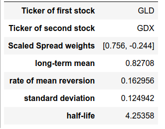
To view the estimated model parameters from training data, call the describe function.

OUModelJurek.describe() → Series

Method returns values of instance attributes calculated from training data.

Returns:

(pd.Series) Series describing parameter values.

Step 2: Getting the Optimal Portfolio Weights

In this step we input the evaluation data and specify the type of investor we are looking for. We also need to specify the utility function parameter \(\gamma\) and the risk free rate of return \(r\).

If we choose the investor with intermediate consumption, we also need to specify the parameter \(\beta\).

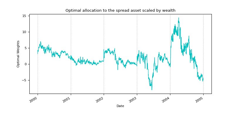
An example showcasing the optimal allocation to the spread asset (in cyan) scaled by wealth, \(N_t/W_t\). In the out-of-sample trading simulation the agent uses a fixed length backward-looking window to estimate the parameters of the model, and uses those estimates to trade in the test window. For the plots in this doc, five test windows are shown.

Implementation

OUModelJurek.optimal_portfolio_weights(prices: DataFrame, utility_type: int = 1, gamma: float = 1, beta: float = 0.01, r: float = 0.05) → array

Implementation of Theorem 1 and Theorem 2 in Jurek (2007).

This method implements the optimal portfolio strategy for two types of investors with varying utility functions.

The first type of investor is represented by utility_type = 1. This agent has constant relative risk aversion preferences(CRRA investor) with utility defined over terminal wealth. For this type of investor,

gamma = 1 implies log utility investor, and gamma != 1 implies general CRRA investor.

The second type of investor is represented by utility_type = 2. This agent has utility defined over intermediate consumption, with agent’s preferences described by Epstein-Zin recursive utility with psi(elasticity of intertemporal substitution) = 1. For this type of investor,

gamma = 1 reduces to standard log utility investor, and gamma > 1 implies more risk averse investors, whereas gamma < 1 implies more risk tolerance in comparison to investor with log utility.

What is beta? Beta signifies the constant fraction of total wealth an investor chooses to consume. This is analogous to a hedge fund investor who cares both about terminal wealth in some risk-averse way and consumes a constant fraction, β, of assets under management (the management fee). For utility_type = 2, C(Consumption) = beta * W.

Parameters:

• prices – (pd.DataFrame) Contains price series of both stocks in spread.

• utility_type – (int) Flag signifies type of investor preferences. (Either 1 or 2).

• gamma – (float) coefficient of relative risk aversion. (gamma > 0).

• beta – (float) Subjective rate of time preference. (Only required for utility_type = 2).

• r – (float) Rate of Returns. (r > 0).

Returns:

(np.array) Scaled optimal portfolio weights.

Note

The output of the optimal_portfolio_weights method is the portfolio weights of the spread scaled w.r.t wealth.

Tip

The spread_calc method can be used to calculate the spread on the test data.

OUModelJurek.spread_calc(prices: DataFrame) → tuple

This method calculates the spread on test data using the scaled weights from training data.

Parameters:

prices – (pd.DataFrame) Contains price series of both stocks in spread.

Returns:

(tuple) Consists of time remaining array and spread numpy array.

Step 3: Stabilization Region

In this optional step, we can calculate the boundaries of the stabilization region for the spread calculated from the data.

Implementation

OUModelJurek.stabilization_region(prices: DataFrame, utility_type: int = 1, gamma: float = 1, beta: float = 0.01, r: float = 0.05) → tuple

Implementation of Theorem 3 in Jurek (2007).

Parameters:

• prices – (pd.DataFrame) Contains price series of both stocks in spread.

• utility_type – (int) Flag signifies type of investor preferences.

• gamma – (float) coefficient of relative risk aversion.

• beta – (float) Subjective rate of time preference. (Only required for utility_type = 2).

• r – (float) Rate of Returns.

Returns:

(tuple) Tuple of numpy arrays for spread, min bound and max bound.

An example showcasing the evolution of the Royal Dutch - Shell spread asset (in cyan), \(S_t\), within each trading period, and the corresponding stabilization bound (in red).

Step 4: Optimal Portfolio Weights with Fund Flows

In this optional step, we calculate the optimal portfolio weights with the inclusion of fund flows for the CRRA investor.

Implementation

OUModelJurek.optimal_portfolio_weights_fund_flows(prices: DataFrame, f: float, gamma: float = 1, r: float = 0.05) → array

Implementation of Theorem 4 in Jurek (2007).

This method calculates the optimal portfolio allocation of an agent with constant relative risk aversion with utility defined over terminal wealth, (utility_type = 1) , in the presence of fund flows.

Note: For all values of gamma, the presence of fund flows affect the general portfolio rule only by introducing a coefficient of proportionality.

Also note, this method is only applicable for investors with utility defined over terminal wealth.

What is f?

f is the coefficient of proportionality for fund flows and is the drift term in the stochastic process equation for fund flows. (Refer Appendix C)

Parameters:

• prices – (pd.DataFrame) Contains price series of both stocks in spread.

• gamma – (float) coefficient of relative risk aversion. (gamma > 0).

• f – (float) coefficient of proportionality (f > 0).

• r – (float) Rate of Returns. (r > 0).

Returns:

(np.array) Optimal weights with fund flows.

Note

The output of the optimal_portfolio_weights_fund_flows method is the portfolio weights of the spread scaled w.r.t wealth.

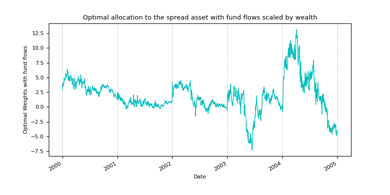
An example showcasing the optimal allocation to the spread asset (in cyan) scaled by wealth, \(N_t/W_t\), for the case with fund flows.

Step 5: Plotting

In this optional step, we can plot the stabilization region, optimal portfolio weights and the evolution of wealth.

Implementation

OUModelJurek.plot_results(prices: DataFrame, num_test_windows: int = 5, delta_t: float = 0.003968253968253968, utility_type: int = 1, gamma: float = 10, beta: float = 0.01, r: float = 0.05, f: float = 0.1, figsize: tuple = (8, 4), fontsize: int = 8)

Method plots out of sample performance of the model on specified number of test windows. We use a backward looking rolling window as training data and its size depends on the number of test windows chosen. The length of training data is fixed for all test windows.

For example, if the total data is of length 16 years, with the number of test windows set to 5, the length of training data would be 16 - (5 + 1) = 10. (The last year is not considered for testing).

This method plots the stabilization region, optimal portfolio weights with and without fund flows, and the evolution of the wealth process with initial wealth normalized to 1.

Parameters:

• prices – (pd.DataFrame) Contains price series of both stocks in spread with dates as index.

• num_test_windows – (int) Number of out of sample testing windows to plot.

• delta_t – (float) Time difference between each index of prices, calculated in years.

• utility_type – (int) Flag signifies type of investor preferences.

• gamma – (float) coefficient of relative risk aversion.

• beta – (float) Subjective rate of time preference. (Only required for utility_type = 2).

• r – (float) Rate of Returns.

• f – (float) Coefficient of proportionality (assumed to be positive).

• figsize – (tuple) Input to matplotlib figsize parameter for plotting.

• fontsize – (int) general matplotlib font size for plotting.

Examples

We use GLD and GDX tickers from Yahoo Finance as the dataset for this example.

import yfinance as yf

data1 =  yf.download("GLD GDX", start="2009-03-25", end="2019-03-25")
data2 =  yf.download("GLD GDX", start="2019-03-27", end="2020-03-27")

data_train_dataframe = data1["Adj Close"][["GLD", "GDX"]]
data_test_dataframe = data2["Adj Close"][["GLD", "GDX"]]

Note

To get good results for the estimated parameters, using t 10 years of training data is recommended.

Example 1

In the following code block, after initializing the class firstly, we use the fit method to generate the parameters of the model. Then, we call describe to view the estimated parameters. Finally, we use the out-of-sample test data to calculate the optimal portfolio weights using the fitted model.

from arbitragelab.stochastic_control_approach.ou_model_jurek import OUModelJurek

sc = OUModelJurek()

sc.fit(data_train_dataframe)

print(sc.describe())

plt.plot(sc.optimal_portfolio_weights(data_test_dataframe, beta=0.01, gamma=0.5, utility_type=1))
plt.show()

Warning

For utility_type = 2 and low values of \(\gamma (< 1)\), the model becomes unstable with respect to the value of \(k\).

Example 2

In the following code block, after initializing the class firstly, we use the fit method to generate the parameters of the model. Then, we call describe to view the estimated parameters. Finally, on the out-of-sample test data we calculate the stabilization region for the spread calculated from test data.

from arbitragelab.stochastic_control_approach.ou_model_jurek import OUModelJurek

sc = OUModelJurek()

sc.fit(data_train_dataframe)

print(sc.describe())

S, min_bound, max_bound = sc.stabilization_region(data_test_dataframe, beta=0.01, gamma=0.5, utility_type=1)

plt.plot(S, label='Spread')
plt.plot(min_bound, color='red', linestyle='dashed')
plt.plot(max_bound, color='red', linestyle='dashed')
plt.legend()
plt.show()

Example 3

In the following code block, after initializing the class firstly, we use the fit method to generate the parameters of the model. Then, we call describe to view the estimated parameters. Finally, we use the out-of-sample test data to calculate the optimal portfolio weights with fund flows using the fitted model.

from arbitragelab.stochastic_control_approach.ou_model_jurek import OUModelJurek

sc = OUModelJurek()

sc.fit(data_train_dataframe)

print(sc.describe())

plt.plot(sc.optimal_portfolio_weights_fund_flows(data_test_dataframe, f=0.05, gamma=0.5))
plt.show()

Research Notebook

The following research notebook can be used to better understand the approach described above.

• Dynamic Portfolio Selection in Arbitrage

Download Notebook Download Sample Data

Research Article

Read our article on the topic

Presentation Slides

References

• Jurek, J.W. and Yang, H., 2007, April. Dynamic portfolio selection in arbitrage.